Next: 3 Further Operations and
Up: 5 Applications of Matrix
Previous: 1 Calculation of Covariance
Index
2 Transformations of Data Matrices
Matrix algebra provides a natural notation for transformations.
If we premultiply the matrix
 by another, say
 , then the rows of
  describe linear
combinations of the rows of
describe linear
combinations of the rows of  . The resulting matrix will
therefore consist of
. The resulting matrix will
therefore consist of  rows corresponding to the linear
transformations of the rows of
rows corresponding to the linear
transformations of the rows of  described by the rows of . A very simple example of this is premultiplication by the
identity matrix, I, which, as noted earlier, merely has 1's on
the leading diagonal and zeroes everywhere else. Thus, the
transformation described by the first row may be written as `multiply
the first row by 1 and add zero times the other rows.' In the second
row, we have `multiply the second row by 1 and add zero times the
other rows,' and so the identity matrix transforms the matrix B
into the same matrix. For a less trivial example, let our data matrix
be
described by the rows of . A very simple example of this is premultiplication by the
identity matrix, I, which, as noted earlier, merely has 1's on
the leading diagonal and zeroes everywhere else. Thus, the
transformation described by the first row may be written as `multiply
the first row by 1 and add zero times the other rows.' In the second
row, we have `multiply the second row by 1 and add zero times the
other rows,' and so the identity matrix transforms the matrix B
into the same matrix. For a less trivial example, let our data matrix
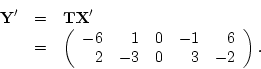
be  , then
and let
then
In this case, the transformation matrix specifies two transformations
of the data: the first row defines the sum of the two variates, and
the second row defines the difference (row 1  row 2). In the
above, we have applied the transformation to the raw data, but for
these linear transformations it is easy to apply the transformation to
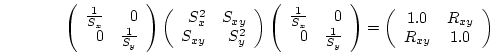
the covariance matrix. The covariance matrix of the transformed
variates is
row 2). In the
above, we have applied the transformation to the raw data, but for
these linear transformations it is easy to apply the transformation to
the covariance matrix. The covariance matrix of the transformed
variates is
which is a useful result, meaning that linear transformations may be
applied directly to the covariance matrix, instead of going to the
trouble of transforming all the raw data and recalculating the
covariance matrix.
Next: 3 Further Operations and
Up: 5 Applications of Matrix
Previous: 1 Calculation of Covariance
Index
Jeff Lessem
2002-03-21