Michael C. Neale
Mx:
Statistical Modeling
by
Michael C. Neale
Department of Psychiatry, Virginia Institute for Psychiatric and Behavioral Genetics,
Virginia Commonwealth University, Richmond, Virginia, U.S.A.
Steven M. Boker
Department of Psychology,
University of Notre Dame, Notre Dame, Illinois, U.S.A.
Gary Xie
Department of Psychiatry, Virginia Institute for Psychiatric and Behavioral Genetics,
Virginia Commonwealth University, Richmond, Virginia, U.S.A.
Hermine H. Maes
Department of Human Genetics, Virginia Institute for Psychiatric and Behavioral Genetics, Virginia Commonwealth University, Richmond, Virginia, U.S.A.
Virginia Institute for Psychiatric and Behavioral Genetics
Virginia Commonwealth University
Department of Psychiatry
First Published 1991
Second Edition 1994
Third Edition 1995
Fourth Edition 1997
Draft Fifth Edition 1999
Refer to Mx manual as:
Neale MC, Boker SM, Xie G, Maes HH (1999). Mx: Statistical Modeling. Box 126 MCV, Richmond, VA 23298: Department of Psychiatry. 5th Edition.
All rights reserved
© 1999 Michael C. Neale
List of Tables 11
List of Figures 13
Preface 15
1 Introduction to
Structural Equation Modeling 1
1.1 Guidelines for good Script Style 1
1.2 Matrix Algebra 1
1.3 Structural Equation Modeling 2
RAM Approach 2
Simplified Mx Approach 6
Fully Multivariate Approach 8
1.4 Other Types of Statistical Modeling 10
2 Introduction to the
Mx Graphical User Interface
11
2.1 Using Mx GUI 11
2.2 Fitting a Simple Model 12
Preparing the Data 12
Drawing the Diagram 12
Fitting the Model 13
Viewing Results 13
Saving Diagrams 16
2.3 Revising a Model 16
Adding a Causal Path 16
Adding a Covariance Path 16
Changing Path Attributes 17
Fixing a Parameter 18
Confidence Intervals 18
Equating Paths 18
Moving Variables and Paths 19
2.4 Extending the Model 19
Multiple Groups: Using Cut and Paste 19
Selecting Different Variables for Analysis 22
Modeling Means 22
2.5 Output Options 23
Zooming in and out 23
Copying Matrices to the Clipboard 24
Comparing Models 24
Setting Job Options 24
Printing 26
Exporting Diagrams to other Applications 27
Files and Filename Extensions 28
2.6 Running Jobs 28
Running Scripts 28
Using Networked Unix Workstations 29
2.7 Advanced Features 31
Adding Non-linear Constraints to Diagrams 31
Moderator Variables: Observed Variables as Paths 33
3 Outline of Mx Scripts and Data Input 36
3.1 Preparing Input Scripts 36
Comments, Commands and Numeric Input 36
Syntax Conventions 36
Job Structure 37
Single Group Example 38
#Define Command 39
Matrices Declaration 40
Matrix Algebra 40
3.2 Group Types 41
Title Line 41
Group-type Line 41
3.3 Commands for Reading Data 42
Covariance and Correlation Matrices 42
Asymptotic Variances and Covariances 42
Variable Length, Rectangular and Ordinal Files 43
Missing Command 45
Definition Variables 45
Contingency Tables 45
Means 46
Higher Moment Matrices 46
3.4 Label and Select Variables 46
Labeling Input Variables 46
Select Variables 47
Select If 47
3.5 Calculation and Constraint Groups 48
Calculation Groups 48
Constraint Groups 48
4 Building Models with Matrices 50
4.1 Commands for Declaring Matrices 50
Matrices Command 50
Matrix Types 51
Equating Matrices across Groups 51
Free Keyword 52
4.2 Building Matrix Formulae 54
Matrix Operations 54
Matrix Functions 58
4.3 Using Matrix Formulae 67
Covariances, Compute Command 67
Means Command 67
Threshold Command 68
Weight command 68
Frequency Command 69
4.4 Putting Numbers in Matrices 70
Matrix Command 70
Start and Value Commands 71
4.5 Putting Parameters in Matrices 72
Pattern Command 72
Fix and Free Commands 72
Equate Command 73
Specification Command 74
Boundary Command 74
4.6 Label Matrices and Select Variables 75
Labeling Matrices 75
Identification Codes 75
5 Options for Fit Functions andOutput 78
5.1 Options and End Commands 78
5.2 Fit Functions: Defaults and Alternatives 78
Standard Fit Functions 79
Maximum Likelihood Analysis of Raw Continuous Data 81
Maximum Likelihood Analysis of Raw Ordinal Data 82
Contingency Table Analysis 84
User-defined Fit Functions 85
5.3 Statistical Output and Optimization Options 86
Standard goodness-of-fit output 86
RMSEA 86
Suppressing Output 87
Appearance 87
Residuals 87
Adjusting Degrees of Freedom 88
Power Calculations 88
Confidence Intervals on Parameter Estimates 89
Standard Errors 91
Randomizing Starting Values 91
Automatic Cold Restart 92
Jiggling Parameter Starting Values 92
Confidence Intervals on Fit Statistics 92
Comparative Fit Indices 93
Automatically Computing Likelihood-Ratio Statistics of Submodels 93
Check Identification of Model 94
Changing Optimization Parameters 94
Setting Optimization Parameters 95
5.4 Fitting Submodels: Saving Matrices and Files 96
Fitting Submodels using Multiple Fit Option 96
Dropping Parameters from Model 98
Reading and Writing Binary Files 98
Writing Matrices to Files 99
Formatting and Appending Matrices Written to Files 99
Writing Individual Likelihood Statistics to Files 100
Creating RAMpath Graphics Files 101
6 Example Scripts 102
6.1 Using Calculation Groups 102
General Matrix Algebra 102
Assortative Mating 'D' Matrix 102
Pearson-Aitken Selection Formula 104
6.2 Model Fitting with Genetically Informative Data 105
ACE Genetic Model for Twin Data 105
Power Calculation for the Classical Twin Study 106
RAM Specification of Model for Twin Data 109
Cholesky Decomposition for Multivariate Twin Data 111
PACE Model: Reciprocal Interaction between Twins 113
Scalar, Non-scalar Sex Limitation and Age Regression 115
Multivariate Assortative Mating: Modeling D 118
6.3 Fitting Models with Non-linear Constraints 118
Principal Components 118
Analysis of correlation matrices 119
Fitting a PACE Model to Contingency Table Data 121
Twins and their Parents: Cultural and Genetic Transmission
122
6.4 Fitting Models to Raw Data 130
Estimating Means and Covariances 130
Variable Pedigree Sizes 131
Definition Variables 132
Using NModel to assess heterogeneity 134
Least Squares 138
Correction for Ascertainment 139
A Using Mx under different operating systems 142
A.1 Obtaining Mx 142
A.2 System Requirements 142
A.3 Installing the Mx GUI 142
A.4 Using Mx 142
B Error Messages 146
B.1 General Input Reading 146
B.2 Error Codes 146
C Introduction to Matrices 154
C.1 The Concept of a Matrix 154
C.2 Matrix Algebra 155
Transposition 155
Matrix Addition and Subtraction 155
Matrix Multiplication 156
C.3 Equations in Matrix Algebra 159
C.4 Calculation of Covariance Matrix from Data Matrix 160
Transformations of Data Matrices 162
Determinant of a Matrix 163
Inverse of a Matrix 164
D Reciprocal Causation 168
E Frequently Asked Questions 172
References 174
Index 180
2.1 Correspondence between optimization codes and IFAIL parameter 13
2.2 Summary of filename extensions used by Mx 28
3.2 Parameters of the group-type line 41
4.1 Matrix types 51
4.2 Syntax for constraining matrices to special quantities 52
4.3 Examples of use of the Matrices command 53
4.4 Matrix operators 54
4.5 Matrix functions 59
5.1 Default fit functions 79
6.1 Summary of parameter estimates for a variety of models of heterogeneity 135
1.1 Example path diagram 3
1.2 Multivariate path diagram 7
2.1 Mx GUI with Project Manager Window 11
2.2 The Results Panel 13
2.3 The Results Box Panel 14
2.4 Mx Path Inspector 17
2.5 Starting values for an ACE twin model for MZ twins 21
2.6 Parameter estimates from fitting the ACE model 21
2.7 The Job Option Panel 25
2.8 Host Options Panel 30
2.9 Higher Order Factor Model 31
2.10 Linear Regression with Interaction Model 34
2.11 Linear Regression with Interaction 35
3.1 Factor model for two variables 38
5.2 Contour plot showing a bivariate normal distribution 84
6.1 ACE genetic model for twin data 105
6.2 Cholesky or triangular factor model 111
6.3 PACE model for phenotypic interaction 113
6.4 Model for sex limitation and age regression 115
6.5 Three factor model of 9 cognitive ability tests 120
6.6 Model of mixed genetic and cultural transmission 123
6.7 Definition variable example 133
C.1 Graphical representation of the inner product 157
C.2 Geometric representation of the determinant 163
D.1 Feedback loop between two variables 168
D.2 Structural equation model for x variables 169
D.3 Structural equation model for y variables 170
What Mx does
Mx is a structural equation modeling package, but it is flexible enough to fit a variety of other mathematical models. At its heart is a matrix algebra processor, which can be used by itself. There are many built-in fit functions to enable structural equation modeling and other experiments in matrix algebra and statistical modeling. It offers the fitting functions found in commercial software such as LISREL, LISCOMP, EQS, SEPATH, AMOS and CALIS, including facilities for maximum likelihood estimation of parameters from missing data structures, under normal theory. Complex 'nonstandard' models are easy to specify. For further general applicability, it allows the user to define their own fit functions, and optimization may be performed subject to linear and nonlinear equality or boundary constraints.
How to Read this Manual
The bad news is that this manual is quite long; the good news is that you don't need to read it all! Chapter 1 contains an introduction to multivariate path modeling. The "how to" part of the manual starts in Chapter 3, in which general syntax conventions and job structure are laid out, followed by description of the commands necessary to read data. Chapter 4 deals with the heart of Mx: how to define matrices and matrix algebra formulae for model-fitting, and ways of estimating and constraining parameters. Methods of changing the default fit-function, of decreasing and increasing the quantity (and quality) of the output, and for fitting sub-models efficiently, are described in Chapter 5. The last chapter supplies and briefly describes a number of example scripts. The Appendices describe the use of Mx under different operating systems, error codes, introductory matrix algebra and reciprocal causation.
Origin
The development of Mx owes much to LISREL and I acknowledge the pioneering effort put in by Karl Jöreskog & Dag Sörbom. There are many who have supported and encouraged this effort in many different ways. I thank them all, and especially Lindon Eaves, Ken Kendler and John Hewitt since they also provided grant support(1), and David Fulker for allowing modification of his notes on matrix algebra to be supplied as an appendix to this manual. Jack McArdle and Steve Boker provided excellent path diagram drawing software (RAMPATH) which was the basis for the development of Mx Graph, Luther Atkinson suggested the binary file save option; Buz Brown programmed the Rectangular file read, Karen Kenny and John Fritz organized the interactive website; these efforts were part of the excellent software, hardware and consultancy support supplied by University Computing Services at the Medical College of Virginia, Virginia Commonwealth University. The Mx team includes my colleagues Drs. Steve Boker, Hermine Maes, Mr. Gary Xie and Wayne Hadady.
What's New in 1999
New in this edition is the Mx Graphical interface documentation. Chapter 2 describes how to take advantage of this software which is available for the MS Windows (Win3.x/98/NT) platform. Jobs built with diagrams or scripts can be executed on a Unix server to get results more quickly for CPU intensive modeling.
Several features have been added to enable modeling ordinal data. P ? is the ordinal file command, which operates like a rectangular file read except that it expects ordinal data with a lowest category of zero. Likelihoods are then computed using numerical integration software provided by Genz (1992). The same software is used in the latest function which returns all of the cell proportions for a covariance matrix and set of thresholds.
A new frequency command (described on p ?) supplements the weight command by allowing different cases to have different weights. This feature allows data-weighting approaches to be implemented.
A number of new features improve the quantity and quality of statistical and matrix output. First, the difference between a supermodel and a submodel can be computed automatically if the option Issat is used to identify a supermodel, or if option sat is used to enter the fit of a supermodel against which new models are to be compared. Matrix output can be formatted with any legal Fortran format, and matrices written can be appended to existing files. This latter feature is useful for simulation work because the results of several model-fitting runs can be written to the same file for later analysis.
Several new examples have been added, both to the text and to the Mx website. It is a pleasure to continue to offer Mx free of charge, which allows rapid fixing of bugs and immediate release of new features.
Internet Support
Mx is public domain; it is available from the internet at http://griffin.vcu.edu/mx/. With a suitable browser, you can obtain the program, documentation and examples, send comments, see the latest version available for your platform, and so on. E-mail bug reports, requests for further information, and most important your comments and suggestions for improvements to neale@psycho.psi.vcu.edu - it is hard to overemphasize the importance of constructive criticism. You can also grab the code for a variety of operating systems via anonymous ftp to opal.vcu.edu. Please have the courtesy (and self-interest) to E-mail me so that I can keep you informed of updates, bug reports etc.
A graphical interface for structural equation modeling, "Mx Graph" is currently in alpha-test to Mx that will relieve the user of getting to grips with the details of scripts. Even with this interface, knowledge of the script language is necessary to use advanced features and methods. The good news is that a much deeper understanding of modeling can come from this activity. We are in the process of revising the script language to enhance its flexibility and readability.
Technical Support
A number of users have been most helpful finding errors in the documentation or software or both, and for suggesting new features that would make Mx easier to use. Thank you! I hope that all users will forward any comments, bug reports, or wish-lists to me. My current address is:
address Department of Psychiatry
Virginia Institute for Psychiatric and Behavioral Genetics
Box 126 MCV
Richmond VA 23298-0126, USA
phone 804 828 3369
fax 804 828 1471
E-mail neale@psycho.psi.vcu.edu (internet)
and my order of preference for communication is E-mail, fax, phone and snail mail. When reporting problems, E-mail is especially useful to include the problem file.
| To find | Go to |
| Matrix Algebra
Learn basic Syntax |
Appendix C |
| SEM Path Analysis | Neale & Cardon (1992) chapter 5
Loehlin (1987) McArdle & Boker (1990) Everitt (1984) |
| How to do basic SEM | Chapter 1 |
| How to recast basic SEM
more efficiently |
Chapter 1 |
| How to use the graphical interface | Chapter 1 |
| Job Structure | Chapter 3 |
| Reading Data | Chapter 3 |
| Declare Matrices
Use Matrix Formulae |
Chapter 4 |
| Use different Fit Functions,
Write Output to Files Change Options |
Chapter 5 |
| Look through Example Scripts | Chapter 6 |
| Quick Check of Syntax | Index
Quick Reference Guide |
| Operating Systems | Appendix A |
| Icons | Meaning |
| Caution | |
| Note | |
| Efficiency tip |
What you will find in this chapter
1.1 Guidelines for good Script Style
Programming, like much of life, requires compromises. We must balance the time taken to do things against their value. Now, there are both short-term considerations ("how do I get this working as soon as possible?") and long-term ones ("how can I save time in what I'm going to be doing next week?"). This usually results in making a choice of method that is based on the following factors:
Normally, we would choose a method that will solve our problem in the shortest time. If we expect to use the same basic model but with a varying number of observed and latent variables, then it is worth spending the extra time to write a script in which these changes can be made easily.
Part of writing good scripts is to write them so that you, or colleagues can understand them. Sometimes readability can be at the expense of efficiency, and it is up to you to decide on the balance between the two. One of the most important things to remember is to put plenty of comments in your scripts. Doing so can seem like a waste of time, but it usually pays off handsomely when the scripts are read by yourself or others at a later date.
Mx will evaluate matrix algebra expressions. It has a simple language, which uses single letters to represent matrices, certain characters to represent matrix operations, and a special syntax to invoke matrix functions. Thus the program can be used as a matrix algebra calculator, which is helpful in a variety of research and educational settings, and which provides a powerful way to specify structural equation and other mathematical models. Most users of multivariate statistics will need to know some matrix algebra, and Appendix I gives a brief introduction to the subject, along with examples and exercises which use Mx. Even those familiar with matrix algebra should review the "How to do it in Mx" sections in the appendix as that is where elementary principles of writing Mx scripts are introduced.
1.3 Structural Equation Modeling
One of the most common uses of Mx is to fit Structural Equation Models (SEM) to data. A nice aspect of SEM is that the models can be represented as a path diagram. Mx Graph incorporates path diagram drawing software directly; this software is in -test. For now, we concentrate on translating path diagrams into models 'by hand'. This approach has the advantage of giving greater understanding of the modeling process, and can yield highly efficient scripts which are easy to change when, for example, the number of variables changes.
There are many accounts of SEM, which vary widely in complexity and clarity, and which are aimed at different fields of study or different software packages (Jöreskog, K.G. & Sörbom, 1991; Bentler, 1989; Everitt, 1984; Loehlin, 1987; McArdle & Boker 1990; Bollen 1992; Neale & Cardon 1992; Steiger, 1994). The brief account given here is intended to provide a practical guide to setting up models in Mx for those with some familiarity with path analysis or SEM. We begin with a simple, foolproof method, called RAM (McArdle & Boker 1990) which would be ideal except that it is inefficient for the computer to fit. More efficient approaches will follow.
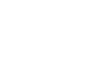
A path diagram consists of four basic types of object: circles, squares, one-headed and two-headed arrows. Circles are used to represent latent (not measured) variables(2), and squares correspond to the observed (or measured) variables. In a path diagram, two types of relationship between variables are possible: causal and correlational. Causal relationships are shown with a one-headed arrow going from the variable that is doing the causing to the variable being caused. Correlational or covariance relationships are shown with two headed arrows. A special type of covariance path is one that goes from the variable to itself. Variation in a variables which is not due to causal effects of other variables in the diagram is represented by this self-correlational path. Sometimes this is called 'residual variance' or 'error variance'.
Figure 1.1 shows a sample path diagram with two latent variables and four observed. The
RAM model specification involves three matrices: F, A and S. S is for the symmetric paths,
or two-headed arrows, and is symmetric. A is for the asymmetric paths, or one-headed
arrows, and F is for filtering the observed variables out of the whole set. The dimensions
of these matrices are fixed by the number of variables in the model. A and S are both m�m,
and F is mO�m, where m=mO+mL is the total number of variables in the model, ![]() the
number of observed variables, and
the
number of observed variables, and ![]() the number of latent variables. In our example we
have mO=4, mL=2 and m=6.
the number of latent variables. In our example we
have mO=4, mL=2 and m=6.


Now that we have defined these matrices, computing the predicted covariance matrix under this model is relatively simple. The formula is:
!
! Simple RAM approach to fitting models
!
#Ngroups 1
#define latent 2 ! Number of latent variables
#define meas 4 ! Number of measured variables
#define m 6 ! Total number of variables, measured + latent
Title Ram approach to fitting models ! Title
Data NInput=meas NObserved=100 ! Number of variables,subjects
CMatrix File=ramfit.cov ! Reads observed covariance matrix
Matrices; ! Declares matrices
A Full m m ! One-headed paths
S Symm m m ! Two-headed paths
F Full meas m ! Filter matrix
I Iden m m ! Identity matrix
End Matrices; ! End of matrix declarations
Specify A ! Set certain elements of A as free parameters
0 0 0 0 0 0
0 0 0 0 0 0
1 0 0 0 0 0
2 0 0 0 0 0
0 3 0 0 0 0
0 4 0 0 0 0
Specify S ! Set the free parameters in S
0
5 0
0 0 6
0 0 0 7
0 0 0 0 8
0 0 0 0 0 9
Value 1.0 S 1 1 S 2 2 ! Put 1's into certain elements of S
Matrix F ! Do the same for Matrix F but a different way
0 0 1 0 0 0 ! Note - this could be omitted if F had
0 0 0 1 0 0 ! been declared ZI instead of full.
0 0 0 0 1 0
0 0 0 0 0 1
Start .5 All ! Supply .5 starting value for all parameters
Covariance F & ((I-A)~ & S); ! Formula for model
End group
This script is organized into six sections: (i) defines, (ii) title and data reading, (iii) declaring matrices, (iv) putting parameters into matrices, (v) putting numbers into matrices and (iv) the formula for the model. More detail on all these components can be found in the body of the manual, but let's look at some of the basic features.
*
1.51
.31 1.17
.22 .19 1.46
.11 .23 .34 1.56
where the * indicates free format.
What are the advantages and disadvantages of setting up models with the RAM method? On the positive side, it is extremely simple and general. It doesn't matter if there are feedback loops, everything will be specified correctly (see Appendix D). Of course, some care may be required with the choice of starting values, but we do have a practical method. On the negative side, the covariance statement involves inverting the (I-A) matrix, which will be slow when we have many variables or a slow computer. Many models do not need to use matrix inversion in the covariance statement. In fact, it is only feedback loops which make this necessary; we can therefore seek a simpler, more efficient specification of the model. There are many of these, but we shall be aiming for one that is systematic and straightforward.
Simplified Mx Approach for Models without Feedback Loops
Consider Figure1.1 again. It has two levels of variables: P and Q at level 1, and R, S, T and U at level 2. We could put all the two-headed arrows at the first level in one matrix, all the level 1 to level 2 arrows in a second matrix, and all the two-headed level 2 arrows in a third matrix. Letting these matrices be X, Y and Z respectively, we would get:


!
! Mx partly simplified approach to fitting models
!
#Ngroups 1
#define top 2 ! Number of variables in top level
#define bottom 4 ! Number of variables in bottom level
Title Mx simplified approach to fitting model ! Title
Data NInput=bottom NObserved=100 ! Number of variables,subjects
CMatrix File=ramfit.cov ! Reads observed covariance matrix
Matrices; ! Declares matrices
X Stan top top free ! Two-headed, top level
Y Full bottom top ! From top to bottom arrows
Z Diag bottom bottom free ! Two-headed, bottom level
End Matrices; ! End of matrix declarations
Specify Y ! Declare certain elements of Y as free parameters
31 0
32 0
0 33
0 34
Start .5 All ! Supply .5 starting value for all parameters
Covariance Y*X*Y' + Z; ! Formula for covariance model
End group
What tricks have we used here? First, the keyword Free in the matrix declaration section makes elements of matrices X and Z free. Matrix X is standardized, which means that it is symmetric with 1's fixed on the diagonal, so free parameter number 1 goes in the lower off-diagonal element (the upper off-diagonal element is automatically assigned this free parameter as well, because standardized matrices are symmetric). Matrix Z is diagonal, so it will have parameters 2 through 5 assigned to its diagonal elements. We could put parameters 6 through 9 in matrix Y, but 31 to 34 are used instead, just to emphasize that we don't want our specification numbers to overlap with specifications automatically supplied by Mx when the free keyword is encountered at matrix declaration time.
Note how this script is much shorter than the original, because of the reduced need for specification statements to put parameters into matrices. This illustrates a valuable feature of programming with Mx: with appropriate matrix formulation of the model, specification statements can be eliminated. The advantage of setting up models in this way is that modifying the model to cater for a different number of observed or latent variables becomes trivially simple. The more complex the model, the greater the value of this approach. Another advantage is that the computer time required to evaluate the model can be greatly reduced. We have not only eliminated the need for matrix inversion when the predicted covariance matrix is being calculated, but also reduced the size of the matrices that are being multiplied.
We now turn to a third implementation of the same model to show how the matrix algebra features can be used to make an efficient script which can be easily modified. Take another look at Figure 1.1. The first latent factor, P, causes the first two observed variables, S and T, whereas the second factor, Q, only affects the other two observed variables, U and V. Perhaps we expect to change the number of observed variables in one or other of these sets. If so, we might want to split the causal paths into two matrices, one for each factor. So, what was matrix Y in the simplified Mx approach will be partitioned into 4 pieces:
We'll use a separate matrix for each of these, and use definition variables to make the changes in their dimensions automatic.
!
! Mx multivariate approach to fitting models
!
#Ngroups 1
#define top 2 ! Number of variables in top level (P,Q)
#define left 2 ! Number of variables in bottom left level (R,S)
#define right 2 ! Number of variables in bottom right level (T,U)
#define meas 4
!
Title Mx simplified approach to fitting model ! Title
Data NInput=meas NObserved=100 ! Number of variables & subjects
CMatrix File=ramfit.cov ! Reads observed covariance matrix
Matrices; ! Declares matrices
X Stan top top free ! Two-headed, top level
J Full left 1 free ! From P to R,S arrows
K Zero left 1 ! From Q to R,S (zeroes)
L Zero right 1 ! From P to T,U (zeroes)
M Full right 1 free ! From Q to T,U arrows
Z Diag meas meas free ! Two-headed, bottom level
End Matrices; ! End of matrix declarations
Start .5 All ! Supply .5 starting value for all parameters
Begin Algebra;
Y = J|K _
L|M ;
End Algebra;
Covariance Y*X*Y' + Z; ! Formula for model
End group
So, the major change here is to use the algebra section to compute matrix Y. We have eliminated the need for a specification statement by applying the keyword free to matrices J and M. If we thought that we might expand the model to have more than one factor for each side, then we could further generalize the script by changing the matrix dimensions from 1 to #define'd variables.
1.4 Other Types of Statistical Modeling
The example in this chapter only deals with fitting a structural equation model to covariance matrices, but Mx will do much more than this! There are many types of fit function built in to handle different types of data for structural equation modeling, including:
Also, the program's multigroup and algebra capabilities cater for tests of heterogeneity, nonlinear equality and inequality constraints, and many other aspects of advanced structural modeling.
Mx has a powerful set of matrix functions and a state-of-the-art numerical optimizer, which make it suitable to implement many other types of mathematical model. One crucial feature makes this possible -- user-defined fit functions. The program will optimize almost anything. Given familiarity with matrix algebra and the basics of Mx syntax, it is often much quicker to implement a new model with Mx than to write a FORTRAN or C program specifically for the task. A slight drawback is that the Mx script may run more slowly than a purpose built programs, although this is usually well worth the saving in development time.
Mx Graphical User Interface
What you will find in this chapter
How to use Mx Graphical User Interface (GUI) to:
Mx GUI can be started by double clicking the Mx icon in either the group window in Windows 3.xx, or from the Start menu in Windows 95. In Windows 95 you may drag the Mx 32 icon from the explorer to the desktop to create a shortcut, which will simplify starting the program.

Figure 2.1 shows a diagram of the layout of the Mx GUI when the Project Manager window is active. The button bar icons are grouped into: filing, editing, printing, running, and drawing. As with any GUI you are free to behave as you like, clicking on buttons in any order. There are, however, some logical ways to proceed that will save time. The purpose of this chapter is to demonstrate the capabilities of the interface and how to use it efficiently.
You can draw path diagrams at any time during an Mx session. A diagram which is either visible in a window or minimized is called open. An Mx script can be automatically created from all open diagrams, sent to the Project Manager, and run. Parameter estimates will be displayed in the diagrams.
Path diagrams are models of latent variables (circles) and observed variables (squares), which are related by causal (one-headed) and covariance (two-headed) paths. While diagrams can be drawn and printed in the abstract, to fit models we must attach or 'map' our data to the squares. Mapping data is the best starting point for drawing a diagram.
We start with a simple dataset: a covariance matrix based on a sample of 123 subjects measured on two variables, X and Y. This information is entered in a .dat file, which for those familiar with Mx notation, contains the Data,CMatrix, and Labels part of an Mx script:
Data Ninput=2 Nobservations=123
CMatrix
.95
.55 1.23
Labels X Y
This file is supplied with Mx Gui; biv.dat was installed in the examples subdirectory of the
Mx installation directory. For details on how to use other types of data, see chapter 3. To
create the file yourself, any text editor, such as Microsoft's Edit program or Notepad will do.
There is a text editor built into the Mx GUI, and by choosing the menu item File|New, or
clicking the new file icon ![]() , a new file can be edited and saved from the File menu or by
clicking the save file
, a new file can be edited and saved from the File menu or by
clicking the save file ![]() . If the file is created with a wordprocessor such as Wordperfect or
Word, it must be saved as ASCII text.
. If the file is created with a wordprocessor such as Wordperfect or
Word, it must be saved as ASCII text.
To start a new diagram, click on the 'new drawing' icon ![]() then click the button marked
then click the button marked
![]() . Then click the biv.dat file to open. The program then shows a list of the
variables in this file. You can highlight one or more of these variables by using click,
shift-click, click and drag, or control-click the usual Microsoft Windows conventions. Get
both X and Y highlighted by positioning the pointer over the X variable, pressing the left
mouse button down, dragging it to the Y variable, and then releasing the mouse button. X
and Y should now be highlighted in blue. Hit
. Then click the biv.dat file to open. The program then shows a list of the
variables in this file. You can highlight one or more of these variables by using click,
shift-click, click and drag, or control-click the usual Microsoft Windows conventions. Get
both X and Y highlighted by positioning the pointer over the X variable, pressing the left
mouse button down, dragging it to the Y variable, and then releasing the mouse button. X
and Y should now be highlighted in blue. Hit ![]() and two new observed variables will
appear in the diagram ready for analysis (they may have appeared behind the data map
window). Click
and two new observed variables will
appear in the diagram ready for analysis (they may have appeared behind the data map
window). Click ![]() to close the data map window.
to close the data map window.
Note that the variables are created with variance paths ![]() (small double-headed arrows).
These paths represent residual variance; they are sometimes called autocorrelational paths.
This is called a 'null model'. It has only variances and no covariances.
(small double-headed arrows).
These paths represent residual variance; they are sometimes called autocorrelational paths.
This is called a 'null model'. It has only variances and no covariances.
Click ![]() to run this job. You will have to supply a job name and a file name. Enter null
for both, without any file extension. Mx GUI will then build, save and run the script file
null.mx. In addition Mx automatically saves the diagram into the file null.mxd which can
be reloaded later.
to run this job. You will have to supply a job name and a file name. Enter null
for both, without any file extension. Mx GUI will then build, save and run the script file
null.mx. In addition Mx automatically saves the diagram into the file null.mxd which can
be reloaded later.
While the job is running, a counter appears. The numbers it displays show that the Mx engine is still trying to solve the problem. When it has finished the message 'Parsing to Core' may appear, indicating that the graphical interface is busy interpreting the results. Often this step is so fast that it is invisible.
After the job has run, the Results Panel appears (see Figure 2.2). It contains information about the status of the optimization; in this example, the words 'Appears OK' should be on the top line, meaning that the solution it found is very likely to be a global minimum(3).

Table 2.1 Correspondence between optimization codes and IFAIL parameter
| Optimization Code | IFAIL | Serious | Action |
| Failed! Incomputable | -1 | Yes | Check output & script for errors |
| Appears OK | 0 or 1 | No | Carefully accept results |
| Failed! Constraint Error | 3 | Yes | Check output & script for
constraint errors |
| Failed! Too few iterations | 4 | Yes | Restart from estimates |
| Possibly Failed | 6 | Sometimes | Restart from estimates |
| Failed! Boundary Error | 9 | Yes | Send script & data to neale@psycho.psi.vcu.edu |
The next line indicates the type of fitting function used, ML ChiSq, which is the usual
Maximum Likelihood fit function for covariance matrices, scaled to yield a 2
goodness-of-fit of the model. The 2 is 39.546 in this example, with lower and upper 90%
confidence intervals of 21.564 and 62.957 respectively. There is one degree of freedom, and
the model fits very poorly (p=.000). There are two free parameters estimated (the two
variance parameters) and three observed statistics (the two variances and the covariance).
Akaike's Information Criterion (AIC) is greater than zero, reflecting poor fit. This
impression is supported by the RMSEA statistic, which should be .05 or less for very good
fit, or between .05 and .10 for good fit. The high value of .538 for RMSEA, and its 90%
confidence intervals which do not overlap regions of good fit (0.393 is greater than .10)
indicate that the model does not fit well. Click on the ![]() to remove the Results Panel. The
Results Panel can be reviewed later by selecting the Output|Fit Results option.
to remove the Results Panel. The
Results Panel can be reviewed later by selecting the Output|Fit Results option.
Viewing Results in the Diagram
When the Results Panel closes, the estimates of the variance parameters for this model become visible in the diagram, on the double-headed arrows. The results panel information has been copied into the diagram. These results can be deleted entirely (click on the results box in the diagram and hit delete or ctrl-x) or the specific elements may be selected for viewing and printing. To display only the fit and p-value we would double click the results box to bring up the results box and change the selections as shown in Figure 2.3. If the null option in the Preferences|Job options panel(see p 24) was used to these data, the grayed-out fit statistics would be available for display in the diagram.

More information about this model can be found in the Project Manager click the
![]() button (or the toolbar icon
button (or the toolbar icon ![]() , to open this window. Highlighted, the script file
name is in the left panel, the group name is in the middle panel, and the first matrix in this
group is in the right hand panel. The values in this matrix are shown in the Matrix
Spreadsheet at the bottom of the Project Manager window.
, to open this window. Highlighted, the script file
name is in the left panel, the group name is in the middle panel, and the first matrix in this
group is in the right hand panel. The values in this matrix are shown in the Matrix
Spreadsheet at the bottom of the Project Manager window.
Fit statistics for the model are shown in the left-hand panel of the manager, F: 39.546 being
the value reported in the Results Panel. You can see the degrees of freedom, df: 1, in the
left-hand Project Manager panel as well, but depending on your display you may have to use
the slider at the bottom of the panel or resize the window to see them. More information on
the fit of the model can be seen in the matrix spreadsheet at the bottom of the Project
Manager by clicking the ![]() button. Click on
button. Click on ![]() again to toggle the view back
to the highlighted matrix.
again to toggle the view back
to the highlighted matrix.
In the middle panel is a list of the groups in the job there's only one group in this case. In
the right hand panel is a list of matrices used to define the model (I, A, F and S), along with
the observed covariance matrix (ObsCov), expected covariance matrix (ExpCov) and the
residual, ObsCov-ExpCov (ResCov). If you click on the ObsCov matrix you can see the
data matrix in the matrix spreadsheet at the bottom of the Project Manager. This view of
the selected matrix can be turned on and off with the ![]() button on the right of the
manager. As described below these matrices can be copied to the cliploard with ctrl-c.
button on the right of the
manager. As described below these matrices can be copied to the cliploard with ctrl-c.
The matrix spreadsheet can show not only the values of the matrix (and its labels) but also
the parameter specifications. If you click on the ![]() button, the parameter specifications
will be shown. Try this out for the S matrix. This is the matrix of Symmetric arrows
(two-headed). There are two of these, one going from X to X and one going from Y to Y.
The free parameters are numbered 1 and 2 in the specs view of the S matrix. A parameter
numbered zero is fixed. The A matrix contains the A symmetric paths (single-headed, causal
arrows) which run from column variable to row variable. There are no causal paths in this
model, so all of the elements of A are zero.
button, the parameter specifications
will be shown. Try this out for the S matrix. This is the matrix of Symmetric arrows
(two-headed). There are two of these, one going from X to X and one going from Y to Y.
The free parameters are numbered 1 and 2 in the specs view of the S matrix. A parameter
numbered zero is fixed. The A matrix contains the A symmetric paths (single-headed, causal
arrows) which run from column variable to row variable. There are no causal paths in this
model, so all of the elements of A are zero.
Click on ExpCov in the right hand panel. To the right is the formula used for this model. Models built from diagrams currently use one general formula for the covariance:
Click on the ResCov matrix in the right hand panel. Notice how the diagonal elements of this matrix are very small. They are presented in scientific notation so 1.23e-08 means .0000000123 and this indicates a good fit of the model to these elements. The model does not fit the off-diagonal elements at all well. It predicts no covariance between these variables, but .55 is quite substantial covariance with this sample size --- as is shown by the fit statistic of 2=39.55 for 1 df. The model should be revised.
The Project Manager window may be resized by pulling the side, top, bottom or corner of
it to a new position. It is also possible to resize the proportion of the window that displays
jobs by dragging(4) the bottom of the group panel up or down to a new position. Also, the
![]() button will switch the matrix spreadsheet on and off.
button will switch the matrix spreadsheet on and off.
All open diagrams are automatically saved to file when the job is run, but sometimes it is useful to save diagrams manually. The null model diagram could be saved directly (without running it) using the following steps:
See page 28 for details on running and saving scripts.
Revising models is easy with the graphical tools.
Returning to the null path diagram, a linear regression model can be devised by adding a
causal path from the independent variable, X, to the dependent variable, Y. It may clarify
the path estimates to put more space between the variables. Click on the open space to
de-select all the variables. Then click on Y and move it a little to the right (if you want to
keep it aligned with X, press shift throughout the operation). Now click on the arrow tool
icon ![]() on the icon bar. In the diagram window, click on X, hold the mouse button down
and drag it to Y, and release the button. The diagram should now have an arrow from X to
Y. Usually we want these arrows to be straight, but sometimes it is useful to make them
curved, which can be done by dragging the little blue square in the middle.
on the icon bar. In the diagram window, click on X, hold the mouse button down
and drag it to Y, and release the button. The diagram should now have an arrow from X to
Y. Usually we want these arrows to be straight, but sometimes it is useful to make them
curved, which can be done by dragging the little blue square in the middle.
You can now hit ![]() in the diagram window. Enter regress for the Job name. Note that
if instead you enter null as the jobname, it will overwrite the previous Mx script and
diagram files. This overwriting approach is useful when trying to get a model correctly
specified initially, but it is better to keep substantively different models in different diagram
and script files. Doing so also allows comparison between them.
in the diagram window. Enter regress for the Job name. Note that
if instead you enter null as the jobname, it will overwrite the previous Mx script and
diagram files. This overwriting approach is useful when trying to get a model correctly
specified initially, but it is better to keep substantively different models in different diagram
and script files. Doing so also allows comparison between them.
The model fits perfectly, as seen by the ML ChiSq of zero in the Results Panel. It also has
zero degrees of freedom, because it has the same number of parameters as it does observed
statistics. Such a model is often called 'saturated'. Click on ![]() to view the new estimates
in the diagram.
to view the new estimates
in the diagram.
The procedure to add a covariance path is essentially the same as for adding a causal path,
but you use the covariance drawing tool instead. Note that there are two types of covariance
path: variance ![]() which appears as a little loop from a variable to itself, and covariance
which appears as a little loop from a variable to itself, and covariance ![]() .
We'll add the covariance type to the diagram.
.
We'll add the covariance type to the diagram.
First, delete the causal path by selecting the pointer tool (the white arrow ![]() ) click on the
path once (a blue dot will appear in the middle of the path to show that it is selected) and
press delete or ctrl-x (cut). Note that you can undo a mistake with the undo tool
) click on the
path once (a blue dot will appear in the middle of the path to show that it is selected) and
press delete or ctrl-x (cut). Note that you can undo a mistake with the undo tool ![]() , and that
tool-changes can be accomplished via a right mouse button click on a diagram.
, and that
tool-changes can be accomplished via a right mouse button click on a diagram.
Second, add the covariance path by selecting the covariance tool ![]() . Then click on X, drag
the pointer to Y, and release. The path is automatically curved a certain amount. The
curvature can be increased or decreased by dragging the blue dot in the middle of the path.
Single-headed arrows can be made to curve in the same way, but their default follows the
convention that they are straight lines, and we recommend keeping them that way if possible
(reciprocal interaction between two variables AB and BA requires some curvature to stop
the lines being on top of each other).
. Then click on X, drag
the pointer to Y, and release. The path is automatically curved a certain amount. The
curvature can be increased or decreased by dragging the blue dot in the middle of the path.
Single-headed arrows can be made to curve in the same way, but their default follows the
convention that they are straight lines, and we recommend keeping them that way if possible
(reciprocal interaction between two variables AB and BA requires some curvature to stop
the lines being on top of each other).
Third, hit ![]() to rerun the model. Enter covar as the name of the job and script. Again
this model fits perfectly, with zero degrees of freedom. The parameter estimates are not all
the same as the regression model we fitted earlier. These two models may be called
'equivalent' because they always explain the data equally well, and a transformation can
be used to obtain the parameter estimates of one model from the other.
to rerun the model. Enter covar as the name of the job and script. Again
this model fits perfectly, with zero degrees of freedom. The parameter estimates are not all
the same as the regression model we fitted earlier. These two models may be called
'equivalent' because they always explain the data equally well, and a transformation can
be used to obtain the parameter estimates of one model from the other.
A variety of characteristics of paths can be changed and made visible in the diagram with the Path Inspector. Double-click the covariance path that we just created in the diagram to bring up the Path Inspector. Using the Inspector a path can be fixed, bounded, or equated to other paths. Confidence intervals can be requested, and the display of labels, start values and other information can be switched on or off. These changes can be made to several paths at once by selecting them all and checking the 'Apply to All Selected' box in the Path Inspector.

For illustration, we will test the hypothesis that the covariance between X and Y is equal to
point two. In the Path Inspector panel for the covariance arrow check () "Fix This
Parameter." Double click the start value field and type in .2 to give the fixed value for this
path. One useful way to remember that a path is fixed is to display only the start value and
not the path label. Uncheck the "Display Label" box and check the "Display Start Value"
box. At the end your Path Inspector panel should look like Figure 2.4. Click OK and then
click ![]() in the diagram window to rerun the model. Enter a new job name such as fixed.
in the diagram window to rerun the model. Enter a new job name such as fixed.
If you now look at the Project Manager and click ![]() , you can see the fit of this model
and compare it with the other models so far. Note that the Path Inspector also allows you to
change the boundaries to restrict path estimates to lie in a particular interval. To constrain
a parameter to be non-negative, we would simply change the lower bound to zero.
, you can see the fit of this model
and compare it with the other models so far. Note that the Path Inspector also allows you to
change the boundaries to restrict path estimates to lie in a particular interval. To constrain
a parameter to be non-negative, we would simply change the lower bound to zero.
For any free parameter you can request confidence intervals. Just double click on the path,
and check the "Calculate CI" and the "Display CI" boxes in the inspector. Run the model
again, but this time just click ![]() without entering a new job name so that the job
overwrites the existing one in the manager. After all, we are fitting the same model and
simply calculating a few more statistics. Mx computes likelihood-based confidence
intervals which have superior statistical properties to the more common type based on
derivatives. Chapter 5 describes the method used, and Neale & Miller (1997) discuss the
advantages of using this type of confidence interval. The main disadvantage is that they are
relatively slow to compute, so we suggest computing them only when the model is finally
correctly specified.
without entering a new job name so that the job
overwrites the existing one in the manager. After all, we are fitting the same model and
simply calculating a few more statistics. Mx computes likelihood-based confidence
intervals which have superior statistical properties to the more common type based on
derivatives. Chapter 5 describes the method used, and Neale & Miller (1997) discuss the
advantages of using this type of confidence interval. The main disadvantage is that they are
relatively slow to compute, so we suggest computing them only when the model is finally
correctly specified.
Mx uses the Labels of the paths to decide whether or not they are constrained to be equal.
To illustrate, add a latent variable to the diagram, and draw causal paths from it to both X
and Y, and constrain the two paths to be equal. First click on the Circle tool ![]() , and click
on the diagram to add the circle. Second, click on the causal path tool and add the two paths
from the new latent variable to X and Y. Third, click on one of the paths and give it the
same label as the other. Finally, to make the model identified we should delete the
covariance (double-headed) path between X and Y. On running it, we should find the same
perfect fit (2=0) of the model. This time we have the square root of the covariance of X
and Y as estimates for the two paths.
, and click
on the diagram to add the circle. Second, click on the causal path tool and add the two paths
from the new latent variable to X and Y. Third, click on one of the paths and give it the
same label as the other. Finally, to make the model identified we should delete the
covariance (double-headed) path between X and Y. On running it, we should find the same
perfect fit (2=0) of the model. This time we have the square root of the covariance of X
and Y as estimates for the two paths.
Note that the latent variable we added had an variance path with the fixed value of 1.00 on it. This is different from the observed variables, which come with free variance paths, corresponding to residual error variance.
Having a fixed variance of 1.00 makes our latent variables standardized by default. Of course, we could make a latent variable unstandardized by fixing it to some other value, or (if there is enough information in the model) estimate its variance as a free parameter.
It is easy to modify the appearance of a diagram by moving one or more variables. To select
a variable, de-select everything by clicking on the selection tool ![]() (5) and then clicking on
some open space in the diagram. Then click on the one variable, and drag it to its new
position. To move several variables together, click on one of them, then press the shift key
and click on another variable. Alternatively, you can click on the background of the diagram
and drag a rectangle around the variables you wish to select. When all the variables to be
moved are selected, you can drag them to their new location.
(5) and then clicking on
some open space in the diagram. Then click on the one variable, and drag it to its new
position. To move several variables together, click on one of them, then press the shift key
and click on another variable. Alternatively, you can click on the background of the diagram
and drag a rectangle around the variables you wish to select. When all the variables to be
moved are selected, you can drag them to their new location.
Multiple Groups: Using Cut and Paste
A valuable feature of graphical interfaces is the ability to rapidly duplicate objects by means of cut and paste. Here we go through a simple multi-group example --- the classical twin study --- to illustrate these actions.
Structural equation modeling of data from twins has been described in detail elsewhere. In summary, twin pairs are diagnosed as either Monozygotic (MZ) or Dizygotic (DZ). The pair is treated as a case, and the MZ pairs are analyzed in a separate group from the DZ. The structural equation model is configured with three latent variables which model possible effects of: additive genes (correlated 1.0 in MZ twins and .5 in DZ pairs); shared environment (correlated 1.0 in both types of twin pair); and individual-specific environment (uncorrelated between twins). This is a two-group example so we will draw two diagrams.
To begin modeling, open the Mx GUI and click on the open a new drawing icon ![]() . Then
click the
. Then
click the ![]() button and the
button and the ![]() button and select the file ozbmiomz.dat from the
examples subdirectory. Select only the variable BMI-T1 and click
button and select the file ozbmiomz.dat from the
examples subdirectory. Select only the variable BMI-T1 and click ![]() to drop it into the
drawing. Move the data map window out of the way or close it, and start working on the
drawing.
to drop it into the
drawing. Move the data map window out of the way or close it, and start working on the
drawing.
We need to add A1, C1 and E1 latent variables. Click on the latent variable icon ![]() and
draw three circles above the BMI-T1 variable. Relabel the variables to read A1, C1 and E1
by double clicking inside the circles and typing in the new text.
and
draw three circles above the BMI-T1 variable. Relabel the variables to read A1, C1 and E1
by double clicking inside the circles and typing in the new text.
Next we need to add the causal paths from A1, C1, and E1 to BMI-T1. Click on the causal
arrow icon ![]() and click and drag from A1 to BMI-T1, and release. Do the same for C1 to
BMI-T1 and E1 to BMI-T1. Mx automatically labels arrows and variables for us, but we
want to use specific names for our paths: a, c and e. Therefore, we double click on each
path in turn and rename it in the label field of the Path Inspector. Care is needed here!
Depending on the order in which the latent variables were drawn, there may already be a
path called a, c or e on one of the latent variables. Relabelling the causal paths may have
inadvertently caused an equality constraint that we don't want. Relabel any of the latent
variable variance paths as necessary to make them different from a, c and e. Finally, because
we are going to model individual-specific variation with e we can remove the variance path
and click and drag from A1 to BMI-T1, and release. Do the same for C1 to
BMI-T1 and E1 to BMI-T1. Mx automatically labels arrows and variables for us, but we
want to use specific names for our paths: a, c and e. Therefore, we double click on each
path in turn and rename it in the label field of the Path Inspector. Care is needed here!
Depending on the order in which the latent variables were drawn, there may already be a
path called a, c or e on one of the latent variables. Relabelling the causal paths may have
inadvertently caused an equality constraint that we don't want. Relabel any of the latent
variable variance paths as necessary to make them different from a, c and e. Finally, because
we are going to model individual-specific variation with e we can remove the variance path ![]() on BMI-T1. Click inside it so that its blue select button appears and hit delete or ctrl-x.
on BMI-T1. Click inside it so that its blue select button appears and hit delete or ctrl-x.
We now have a model for Twin 1, and we need to replicate it for the Twin 2. Either press
ctrl-a or go to the Edit menu and click Select All. Press ctrl-c for copy and ctrl-v for paste
(or use the icons ![]() and
and ![]() or the Edit menu equivalents) and you have a new copy of the
model for an individual. Use the mouse to drag it to the right of the existing model. You
may have to resize the window to give yourself space for this. Alternatively, you can zoom
out the drawing with the
or the Edit menu equivalents) and you have a new copy of the
model for an individual. Use the mouse to drag it to the right of the existing model. You
may have to resize the window to give yourself space for this. Alternatively, you can zoom
out the drawing with the ![]() button (see below).
button (see below).
A very important step comes next. We have duplicated the model for twin 1 --- both the A,
C and E part and the phenotype BMI-T1. We do not want to model the covariance between
BMI-T1 and BMI-T1. When we duplicated the model for twin 1, the new BMI-T1 box was
black rather than blue. This is because it is not mapped to data. To map it, we select the
variable BMI-T1 (and only this variable) in the diagram. Then hit ![]() , click on
BMI-T2 in the variable list, and then
, click on
BMI-T2 in the variable list, and then ![]() . The variable in the diagram turns blue and the
label is revised to say BMI-T2. Mx now knows what data we are analyzing.
. The variable in the diagram turns blue and the
label is revised to say BMI-T2. Mx now knows what data we are analyzing.
To complete the model for MZ twins, we need to do two things. First, change the labels of
the latent variables causing BMI-T2 to A2, C2 and E2 by double clicking on the circles and
typing in the new names. This step is for cosmetic purposes - Mx will still fit the correct
model even if the latent variables have incorrect names. Second, we must specify that the
covariances between A1 and A2 and between C1 and C2 are fixed at one. Click on the
covariance path tool ![]() . Click on A1, drag to A2 and release. Do the same for C1 and C2.
Note that if you drag from right to left, the arrows curve downwards rather than upwards.
The curvature can be adjusted by clicking on the arrow and dragging the blue selection
button in the middle.
. Click on A1, drag to A2 and release. Do the same for C1 and C2.
Note that if you drag from right to left, the arrows curve downwards rather than upwards.
The curvature can be adjusted by clicking on the arrow and dragging the blue selection
button in the middle.
You must now fix the A1-A2 and C1-C2 covariances to one. Click on each path in turn, check the "Fix this parameter" box, make the starting value 1, and select "Display Starting Value". At this stage the diagram should look something like Figure 2.5. It would be possible to run this model, but the parameters a and c are confounded when we have only MZ twins. To identify the model we must add the DZ group.
Adding the DZ twin group is easy. Click on the MZ diagram and hit ctrl-a (select all) and
ctrl-c (copy). Then press the new drawing icon ![]() . Click on the new diagram, press ctrl-v
(paste) and the MZ model is copied into the new drawing window. Two steps remain. First
click on the covariance between A1 and A2 and change its starting value to .5 the value
specified by genetic theory. Second, map the observed variables to data. Hit the
. Click on the new diagram, press ctrl-v
(paste) and the MZ model is copied into the new drawing window. Two steps remain. First
click on the covariance between A1 and A2 and change its starting value to .5 the value
specified by genetic theory. Second, map the observed variables to data. Hit the ![]() button and select the file ozbmiodz.dat. Highlight BMI-T1 and BMI-T2 in the variable list
and click
button and select the file ozbmiodz.dat. Highlight BMI-T1 and BMI-T2 in the variable list
and click ![]() . Because the variable labels in the ozbmiodz.dat file are the same as
the variable labels in the ozbmiomz.dat file, the automap function maps the variables from
the list to the diagram correctly.
. Because the variable labels in the ozbmiodz.dat file are the same as
the variable labels in the ozbmiomz.dat file, the automap function maps the variables from
the list to the diagram correctly.

Fitting the Model
Finally, run the model by clicking the ![]() button in either diagram. Enter ace as the
filename for the script and diagrams. The Results Panel should report a fit of 2.3781 and
the estimates in the diagram should look like those in Figure 2.6.
button in either diagram. Enter ace as the
filename for the script and diagrams. The Results Panel should report a fit of 2.3781 and
the estimates in the diagram should look like those in Figure 2.6.

Note that in this example, there were two Mx errors in the error window. These errors warn us that although we had supplied both means and covariances as data (in the .dat files), only a model for covariances was supplied. See below on page 22 for details on how to graphically model means.
Selecting Different Variables for Analysis
To unmap variables, you must select one and only one variable, go to the data map window,
select only that variable in the list, and then press the ![]() button. You can then remap
the variable in your diagram to another variable in the list by selecting the variable in the list
and pressing
button. You can then remap
the variable in your diagram to another variable in the list by selecting the variable in the list
and pressing ![]() .
.
The ![]() feature lets you automatically map boxes to variables in a dataset by name.
If you have a series of unmapped boxes in your diagram, and a series of unmapped variables
in your dataset, then pressing
feature lets you automatically map boxes to variables in a dataset by name.
If you have a series of unmapped boxes in your diagram, and a series of unmapped variables
in your dataset, then pressing ![]() will map them by name. This is very useful when
you have run an analysis on one dataset, then wish to fit the same model to a different
dataset. It also comes in handy when you have multiple groups, with variables with the
same names being analyzed in different groups, as we did with the twin study example
above.
will map them by name. This is very useful when
you have run an analysis on one dataset, then wish to fit the same model to a different
dataset. It also comes in handy when you have multiple groups, with variables with the
same names being analyzed in different groups, as we did with the twin study example
above.
The Mx GUI allows the user to draw and fit models to means as well as to covariances. This is simplified with a new type of variable in a path diagram, the triangle. Let's add means to the twin model we developed earlier. If you do not still have the MZ and DZ drawings open, load them from the file ace.mxd.
Select the MZ diagram and click on the triangle tool ![]() . Point the mouse somewhere below
the rectangles and click once to create a triangle. Then use the causal path tool
. Point the mouse somewhere below
the rectangles and click once to create a triangle. Then use the causal path tool ![]() to draw
paths from the triangle to the variables BMI-T1 and BMI-T2. Do the same thing in the DZ
group. Mx has automatically set new, free parameters on the paths and we can run the job.
to draw
paths from the triangle to the variables BMI-T1 and BMI-T2. Do the same thing in the DZ
group. Mx has automatically set new, free parameters on the paths and we can run the job.
The output for this job should give exactly the same goodness-of-fit to the model as we had before, because the model for the means is saturated. It has one free parameter for each mean. Let's test the hypothesis that Twin 1 means are equal to Twin 2 means. Go to the MZ diagram and make the label on the path from the triangle to BMI-T1 the same as the label from the triangle to BMI-T2. Do the same in the DZ diagram (keep the labels different from those on the paths from the triangles in the MZ diagram). Run the job again, and give it a new name, like t1eqt2. In the Project Manager window we see that the 2 (F:) has only slightly increased from 2.38 to 2.55 an increase of less than .2 for two degrees of freedom, which is non-significant. This indicates that the hypothesis that the means of twin 1 and twin 2 are equal is not rejected.
To continue the example we can test whether MZ means are equal to DZ means. This is
done by going back to the DZ diagram (ctrl-tab is a shortcut way to switch between Mx
windows) and changing the paths from the triangle so that they have the same label as those
in the MZ group. Run the model again and call it mzeqdz. The 2 of 6.24 has increased by
about 3.7 over the t1eqt2 model, for one degree of freedom, which is not significant at the
.05 level. The hypothesis that the MZ means equal the DZ means is not rejected. The
sample sizes here (637 MZ and 380 DZ pairs) are quite large, so the chance that this result
is a type II error (failure to detect a true effect) is small. The observed MZ-DZ mean
difference must be small relative to the variance of body mass index in these data. We can
check this result in the Project Manager window. Select the t1eqt2 job and examine the
predicted MZ and DZ mean in the ExpMean matrix for the MZ group and compare it with
the ExpMean matrix in the DZ group by alternately selecting the MZ and DZ groups. The
DZ mean is .45 and the MZ mean is .34 which is approximately .11 of a standard deviation
different because the expected variance (see ExpCov) is about .97 for this model. The
standard error of the difference between two means is given by the formula
![]() . This formula isn't entirely appropriate for the case in hand because we
have correlated observations making up the two samples. If we pretend that they are
uncorrelated then the standard error would be approximately 1/760 + 1/1274=.0458. If we
pretend that the twins are perfectly correlated then we would have 1/380 + 1/637=.0648.
The first estimate of the standard error would give a z-score for the difference of
.11/.0458=2.40 (significant at .05 level), whereas the second would give 1.70 (not
significant at .05 level). The truth lies somewhere in between, and a very nice property of
the maximum likelihood testing is that it handles these complications with ease and provides
appropriate tests for both independent and correlated observations. The 2 difference test
above showed that the difference was not quite significant at the .05 level. Better still, we
can obtain confidence intervals on this 2 test and on the parameter estimate itself.
. This formula isn't entirely appropriate for the case in hand because we
have correlated observations making up the two samples. If we pretend that they are
uncorrelated then the standard error would be approximately 1/760 + 1/1274=.0458. If we
pretend that the twins are perfectly correlated then we would have 1/380 + 1/637=.0648.
The first estimate of the standard error would give a z-score for the difference of
.11/.0458=2.40 (significant at .05 level), whereas the second would give 1.70 (not
significant at .05 level). The truth lies somewhere in between, and a very nice property of
the maximum likelihood testing is that it handles these complications with ease and provides
appropriate tests for both independent and correlated observations. The 2 difference test
above showed that the difference was not quite significant at the .05 level. Better still, we
can obtain confidence intervals on this 2 test and on the parameter estimate itself.
The Mx Model for Means
When computing a predicted mean, Mx traces the paths from an observed variable (rectangle) to a mean variable (triangle) and multiplies the paths together. If there are several triangles or pathways from a triangle to an observed variable, it sums their contributions to the mean. Note that, unlike covariances, there is no changing of direction when traversing paths, and only the single-headed arrows are used. The matrix formula Mx uses to compute the predicted means (shown in ExpMean in the Project Manager) is
To zoom into a part of a diagram, click on the zoom in tool ![]() then click on the diagram
workspace and drag a rectangle around the part of the figure that you wish to enlarge.
then click on the diagram
workspace and drag a rectangle around the part of the figure that you wish to enlarge.
To zoom out, select the zoom out tool ![]() click on the diagram and drag a square inside it.
Note that this feature works proportionately, so that it is possible to get a very tiny and
unreadable figure if you drag a very small square by mistake.
click on the diagram and drag a square inside it.
Note that this feature works proportionately, so that it is possible to get a very tiny and
unreadable figure if you drag a very small square by mistake.
Sometimes zooming operations can cause a diagram to become so big or small that it
disappears altogether. A click on the zoom undo button ![]() will shrink or expand the
diagram to roughly fit the window size.
will shrink or expand the
diagram to roughly fit the window size.
Copying Matrices to the Clipboard
A matrix may be copied to the Windows clipboard by selecting it in the right hand panel of
the Project Manager window, and pressing ctrl-c or the copy icon ![]() . The contents of the
windows clipboard may then be pasted into wordprocessing or spreadsheet applications,
usually by pressing ctrl-v or clicking the appropriate paste tool or menu item. By default,
the matrices are copied with a tab character between each column, and a carriage return
character at the end of each row --- suitable for many applications. These defaults may be
changed using Preference|Matrix Options. For example, to obtain output formatted suitable
for a LaTeX table, the user-defined delimiters should be changed to & for columns and \\
for rows. Note also that the number of decimal places may be changed. Diagrams may be
copied to the clipboard as described below.
. The contents of the
windows clipboard may then be pasted into wordprocessing or spreadsheet applications,
usually by pressing ctrl-v or clicking the appropriate paste tool or menu item. By default,
the matrices are copied with a tab character between each column, and a carriage return
character at the end of each row --- suitable for many applications. These defaults may be
changed using Preference|Matrix Options. For example, to obtain output formatted suitable
for a LaTeX table, the user-defined delimiters should be changed to & for columns and \\
for rows. Note also that the number of decimal places may be changed. Diagrams may be
copied to the clipboard as described below.
When several models have been fitted to the same data, it is possible to generate a table of parameter estimates and goodness-of-fit statistics automatically. The menu item Output|Job Compare will build a file of comparisons, which you can view with a text editor. The first column of this file contains a list of all the paths in the model, followed by the fit statistics. The remaining columns are the estimates and fit statistics found for all the models in the project manager. This table may then be copied into other software for publication. The format of the table depends on the Preference|Matrix Options in the same way as copying matrices to the clipboard.
To get only a few of the models in the manager, simply delete the jobs that should be
excluded from the comparison, by selecting them and hitting the Project Manager ![]() button.
button.
Mx uses a default set of job options suitable for most general purpose model-fitting, but there may be times when other settings are desired. The Job Option panel (menu Preference-Job Option) is used to change these settings. Figure 2.7 shows the default settings.

Having run an Mx job, you may wish to view the regular text output. If so, simply hit the
output tool ![]() . The Mx GUI comes with a shareware editor called notebook.exe which you
can select. It allows you to edit and view much larger files than Microsoft Windows'
Notepad editor. You can select an alternative text viewer via Preferences (though we do not
recommend Microsoft Notepad because of its inability to edit large files).
. The Mx GUI comes with a shareware editor called notebook.exe which you
can select. It allows you to edit and view much larger files than Microsoft Windows'
Notepad editor. You can select an alternative text viewer via Preferences (though we do not
recommend Microsoft Notepad because of its inability to edit large files).
Flexview is supplied with Mx to simplify the viewing of HTML output. In order to use it, you must first tell Mx to produce HTML output when it runs, before running the job. This you do via the Preferences-Job Option menu item. Netscape 4.5 could be chosen, but earlier versions start up slowly every time. Under Internet Explorer 4.0, choosing explorer as the html viewer (typically found in c:\windows\explorer.exe) works quite well. For large output files, Flexview does not work well and text output or another viewer should be used. Flexview is shareware and you should register it if you decide to use it regularly.
You can change the number of decimal places and the width of Mx output by entering different values in the decimals and width fields.
Auxiliary output about optimization may be printed to the file nagdump.out by requesting NpSol values greater than 0 (up to 30). Debug output will go to this file as well if Debug is set to 1. Debug prints the values of the parameter estimates and the fit function for each group for every iteration during optimization. Such files can be both large and slow to write to disk, so we recommend only using these features in an emergency.
If you are using raw data, it is possible to save the individual likelihood statistics (see #p. 72) to a file by entering a filename in the text box "Ind. Likelihood File".
Certain 'comparative' fit indices require the computation of the fit of a Null model. By default the null model has free parameters for the variances and zero covariances. This model will be fitted automatically by Mx and the statistics will be computed if the Null model radio button is set to Auto. Sometimes, a different null model than the default is required; this model should be fitted by the user and the 2 and degrees of freedom noted. These statistics would then be entered by first selecting the Manual radio button and then entering values in the Null ChiSq and Null Df fields. The additional statistics will be visible in the Results Panel.
To compute statistical power, the "Power Calculation" checkbox should be checked, and the alpha-level and degrees of freedom should be entered. See the #p. 62 for information on how to fit models that assess statistical power.
By default the Mx GUI requests 90% confidence intervals on fit. If an alternative interval is required, it can be entered in this text field. If CI's are not required, then the check box can be cleared. Note that this is not the same as confidence intervals on the parameter estimates, which must be requested for paths using the Path Inspector.
By default, Mx produces unstandardized parameter estimates. This default may be changed by selecting the "Standardize" check box. The graphical interface then generates different Mx scripts which include non-linear constraint groups to remove the variance of the variables. This box should be checked when working with correlation matrices to obtain correct confidence intervals on the parameters. Correlation matrices should be entered in dat files with a KMatrix not a CMatrix command.
The Restart check box changes the scripts generated from diagrams. Instead of using the starting values of paths, the current estimates are used instead. If a model has been fitted before, and is only slightly changed, e.g. by fixing one parameter, then re-running from the existing estimates may be much faster than starting from the starting values again.
Mx uses certain default values of the optimization parameters which have proven to be reliable under a variety of conditions. Occasionally it is necessary to use different settings; these technical options are described on p. 94. For the most part, these options should not be changed.
If optimization ends with the message "Possibly Failed" you can try to restart optimization automatically with Random Start at -2 for two attempts to solve the problem. If you want to try randomized starting values for a model, set it to a positive value, but be sure to put sensible boundaries on all your free parameters.
To print diagrams, click the printer icon ![]() or use the File menu and select Print. Note that
the part of the diagram visible in the window is printed. Print can also be used to print
scripts from the editor window. The script font can be changed with the Preferences|Script
fonts menu item.
or use the File menu and select Print. Note that
the part of the diagram visible in the window is printed. Print can also be used to print
scripts from the editor window. The script font can be changed with the Preferences|Script
fonts menu item.
Printed output can be previewed with the File|Print preview menu item or the preview tool ![]() on the toolbar. This feature is a good way to save time and paper. Some features of printing,
like printing the object handles on selected objects, may be unexpected, so print preview is
recommended.
on the toolbar. This feature is a good way to save time and paper. Some features of printing,
like printing the object handles on selected objects, may be unexpected, so print preview is
recommended.
There are various ways to improve the visual appearance of the diagrams. Generally, these are worth doing for final copy, such as printing for publication or to make slides for a talk.
First, you can move the path labels away from the paths by clicking on them and dragging them to a new location. Occasionally it may be difficult to select the label because another object, such as the path, is selected instead. If so, try clicking slightly to the right of the label. Second, in Preferences you can choose font size and appearance, separately for the paths and the variables. Also in Preferences you can choose line thickness, which currently affects both the paths and the lines around the variables. To add impact for color printing, you can change the color of the background and foreground components (paths, boxes, text etc.) in a diagram. Third, remember that the amount of information displayed about a path labels, estimates, confidence intervals, boundaries and so on can be changed for individual paths with the Path Inspector. Revising the appearance of many paths simultaneously can be done by selecting several paths and checking the "apply to all" box in the Path Inspector.
The variance arrows sometimes become obscured by paths going to and from variables. They may be dragged to one of eight positions around circles or squares.
Aligning Variables and Paths The grid tool ![]() adds a grid to the currently active
drawing. The color and size of this grid can be changed via the Preferences|Grid menu item.
It is then simple to align circles and squares to this grid by moving them. Much faster is to
use the snap to grid feature
adds a grid to the currently active
drawing. The color and size of this grid can be changed via the Preferences|Grid menu item.
It is then simple to align circles and squares to this grid by moving them. Much faster is to
use the snap to grid feature ![]() , which automatically aligns variables on the grid. Objects
will move only to another grid place, so moving a variable a small distance often won't have
any effect at all. Moving it a greater distance will allow it to snap to a new grid position.
The granularity or size of the grid can be changed using Preferences|Grid size.
, which automatically aligns variables on the grid. Objects
will move only to another grid place, so moving a variable a small distance often won't have
any effect at all. Moving it a greater distance will allow it to snap to a new grid position.
The granularity or size of the grid can be changed using Preferences|Grid size.
Paths labels are given a default central position based on the length and direction of the path
they are labeling. If a path is longer in the vertical axis than the horizontal, its label will be
centered vertically. Conversely, if it is longer in the horizontal axis its label will be centered
horizontally. By moving objects further away it is sometimes possible to automatically align
relevant path labels; this is the preferred way to align path labels. If necessary it is possible
to move each individual label away from its default position by dragging it to a new position
but this should be used as a last resort. We recommend that print preview (File-Print
Preview or ![]() be used to check the visual appearance of a figure.
be used to check the visual appearance of a figure.
Exporting Diagrams to other Applications
Mx GUI uses the standard Windows clipboard to export diagrams to other applications. To
export a diagram, left-click once on the background of the diagram, and then press ctrl-c or
press the copy icon ![]() . This copies the figure to the clipboard. Open another application,
such as Wordperfect, MS Word, Harvard Graphics or Visio and press ctrl-v (or select the
paste menu command or click the paste icon
. This copies the figure to the clipboard. Open another application,
such as Wordperfect, MS Word, Harvard Graphics or Visio and press ctrl-v (or select the
paste menu command or click the paste icon ![]() ). Partial figures may be copied in the same
way, by selecting only part of the diagram before pressing ctrl-c.
). Partial figures may be copied in the same
way, by selecting only part of the diagram before pressing ctrl-c.
Diagrams may also be printed to a postscript file, if you have a postscript printer driver installed. From the printer control menu, select encapsulated postscript as the postscript option, and check the 'Print to file' box.
Mx uses and creates a lot of different files, with specific filename extensions attached to them. To save disk space, some of them may be deleted. Table 2.2 lists the filenames and their contents, and indicates whether they may be safely deleted. Typically one does not want to delete data or useful drawing or script files. Malfunctioning scripts might be better deleted. At this time .prj files cannot be read back into the GUI.
Table 2.2 Summary of filename extensions used by Mx
| File extension | Contents | Delete |
| .dat | Mx data | Probably not |
| .mx | Input script | Probably not |
| .mxd | Mx path diagram | Probably not |
| .mxo | Text output | If no longer needed |
| .htm | Hypertext output | If no longer needed |
| .mxl | Frontend output | Yes |
| .prj | Mx project | Probably not |
| .exe | Executable Mx program | No |
| .dll | Dynamic link library | No |
Many previous users of Mx and those working with non-standard models (such as those involving constraints or special fit functions) will want to be able to run such models. The Mx GUI has been designed to make working with scripts efficient. It lets you open script files, edit them, and view output in either the manager or text or hypertext (HTML) formats. In addition, if there are errors in the script, it will display them and with a click of a button will take you to the editor window with the problem text highlighted.
Let's take an example script. Start the GUI and click the open icon ![]() . Choose twinpar.mx
and hit
. Choose twinpar.mx
and hit ![]() in the editor window. The Mx statistical engine runs the job in the background
and then delivers the output to the manager. We don't need to bother with the details of this
particular job, it's just an example to show how several groups appear. You can easily look
at the matrices in the different groups by selecting the group in the middle panel and the
matrix in the right hand panel.
in the editor window. The Mx statistical engine runs the job in the background
and then delivers the output to the manager. We don't need to bother with the details of this
particular job, it's just an example to show how several groups appear. You can easily look
at the matrices in the different groups by selecting the group in the middle panel and the
matrix in the right hand panel.
As we run more jobs, perhaps editing the script or selecting other scripts, the Project
Manager fills up with the new jobs. The fit statistics from all jobs become visible in the
bottom panel when the ![]() button is pressed.
button is pressed.
Errors in Scripts
To help debugging of Mx scripts, the line and column of the input file where an error occurred is automatically sent to the GUI to speed up debugging of scripts. Let's see how this works with an example.
Edit a dummy script by hitting the new icon ![]() . Type in the following:
. Type in the following:
Title
Data Ngroups=1
Oops a mistake
Begin Matrices;
Hit ![]() and see what happens. Click the left mouse button on the error, and note how the
editor window shows the Oops text highlighted. You are now in a good position to fix the
problem, if you are familiar with the script language. A full description of the language is
given in chapters 3-5 and examples are in chapter 6. Courses on Mx are run quite regularly;
consult http://views.vcu.edu/mx.
and see what happens. Click the left mouse button on the error, and note how the
editor window shows the Oops text highlighted. You are now in a good position to fix the
problem, if you are familiar with the script language. A full description of the language is
given in chapters 3-5 and examples are in chapter 6. Courses on Mx are run quite regularly;
consult http://views.vcu.edu/mx.
Sometimes it is helpful to look at the text or HTML output file to see full details of the error. Click the right mouse button on the error to bring up the output file. With HTML, the error is automatically presented, with Text output it is necessary to scroll to the end of the file.
Using Networked Unix Workstations
Performance and Multi-Platform Environments
The difference in performance between high-end MS windows computers and Unix workstations is narrowing all the time. Indeed, the same hardware can be used for either Unix or MS windows so it might be argued that it has disappeared. However, it is not very cost-effective to supply every student and faculty member with the latest and fastest PC. Many institutions still use a mixed platform computing facility in which there are powerful Unix servers available for general use, along with PC computers that have networked access to these servers. The Unix machines often have large amounts of memory, high-speed disk access and may offer much faster CPU than is available for PC's. To facilitate the use of these remote machines, Mx GUI has a networking component which allows the user to select a remote Unix host to run Mx scripts.
The Host Options Panel
Figure 2.8 shows the Host Options Panel set for local (on the PC on which Mx GUI is running; left panel) and remote processing (right panel). By unchecking the local host checkbox, the user can enter the IP address of the Unix machine and their username and password. Mx is not (yet) a standard part of the Unix operating system, so it must be installed on the host in question before remote access to it will work. The files and instructions for installation are available at http://www.vipbg.vcu.edu/mxgui/unix.html. As a user, you should make sure that your path on the Unix host includes the directory in which Mx-Unix has been installed, which is usually /usr/local/bin.


Figure 2.8 Host Options Panel set for local PC use (left) and remote Unix use (right).
The following steps are required to run a job remotely:
Transferring Files to Unix Hosts
Running Mx GUI on a remote host has a few additional considerations. Foremost is the use
of files, especially the File= subcommand used in Mx scripts. Any file mentioned in a
File= subcommand must be transferred to the remote Unix host (using e.g., ftp) in order for
the Unix host to access it. For this reason, it is best not to put pathnames in the File=
subcommands, because of inconsistencies between the Unix filenaming system and the
windows filenaming system. It would become messy if the only place used for Mx files
was the root directory on the Unix host, so there are facilities for changing directory on the
remote host prior to running scripts there. In the Host Command window, the user can enter
a Unix command such as cd mymxfiles to change directory, before hitting the ![]() .
.
One exception to the need to transfer files to the remote host is the .dat file specified in a
diagram ![]() command. This file will be included in the script and automatically
transferred to the Unix host. For this reason, it can be best to keep all the data in the .dat file
itself and not to use the File= subcommand at all. In some circumstances this may be
inefficient, especially if the network connection is slow, as all the data will be transferred
with the job --- this applies especially to large raw data files or large asymptotic weight
matrices. If several jobs are to be run using the same dataset, it may be more efficient to ftp
these files to the Unix host and return to using File= in the script.
command. This file will be included in the script and automatically
transferred to the Unix host. For this reason, it can be best to keep all the data in the .dat file
itself and not to use the File= subcommand at all. In some circumstances this may be
inefficient, especially if the network connection is slow, as all the data will be transferred
with the job --- this applies especially to large raw data files or large asymptotic weight
matrices. If several jobs are to be run using the same dataset, it may be more efficient to ftp
these files to the Unix host and return to using File= in the script.
The default amount of memory available for the Mx engine to store data, perform matrix algebra and optimization is 100,000 words for the PC version. This can be increased when necessary by changing the value in the Run Options panel (Figure 2.8). The Unix versions have a default of one million words of memory and at present this cannot be altered. If a larger Unix version is required, please email neale@vipbg.vcu.edu for a special build. Sometimes more efficient re-specification of a problem can free up workspace.
In this section we consider some of the more advanced features of Mx GUI, including adding non-linear constraints to diagrams, and the use of continuous moderator variables.
Adding Non-linear Constraints to Diagrams
In earlier sections we saw that it is straightforward to make one path equal another by giving it the same name. It is also simple to force the estimate of a path to lie within certain limits by double-clicking the path and entering boundary constraints. Much less simple is the addition of non-linear constraints which at this time can be done only by directly editing the script.

Figure 2.9 shows a diagram with a higher-order latent factor (H) and two first-order factors F1 and F2. Suppose that we wish to constrain the variance of the second-order factors to equal unity. One simple way to do this might be to eliminate H and allow the factors F1 and F2 to correlate, and give them error components fixed to unity. However, suppose that the paths from H were of substantive interest themselves, perhaps because of reports from other investigations. This example is for illustration, so we'll do it the hard way with non-linear constraints. The data come from Horn & McArdle (1992) and concern the sub-scales of the WAIS intelligence test, taken by subjects aged between 16 and 28 years of age. The tests may be broadly categorized as verbal (IN: Information; CO: Comprehension; SI: Similarities; and VO: Vocabulary) or spatial (PC: Picture Completion; BD: Block Design; PA: Picture Arrangement; and OA: Object Arrangement).
The following steps are necessary:
The most difficult part of the sequence is of course 3(b), where knowledge of the Mx script language and the way that the Mx GUI creates scripts is required. We now give a brief description of the approach used to implement the constraints for this example.
Because the matrix expression for the covariances of all the variables (both latent and observed) is (I-A -1) * S * (I-A-1)' we can compute this by equating matrices to those of the first group, and entering this matrix formula in a Algebra section. More tricky is to extract the relevant matrix elements corresponding to the variances of F1 and F2 This can be achieved using the \part(A,B) function which partitions matrix A according to the rows and columns specified in B. Matrix B must have four elements and these identify two corners of the sub-matrix, so setting the elements of B to 9,9,10,10 will extract the 2�2 matrix from element 9,9 to element 10,10. We know that this is in fact the sub-matrix that we need by looking at the variable labels for matrix S in group 1. Variables F1 and F2 appear as the ninth and tenth elements of the list of labels. A second matrix algebra statement can be used to create the sub-matrix and place it in matrix T.
It remains to equate the diagonal elements of T to unity. This we can do using the d2v matrix function which extracts the diagonal of a matrix to a vector. It is then simple to request a constraint between this vector and a vector in which every element is 1.0, as shown in the following lines of Mx script:
Title Add constraint to variances of F1 and F2
Constraint Ni=2
Begin Matrices = Group 1
P Full 1 4 ! for the partitioning part
U Unit 1 2 ! Two 1.0 elements to equate to variances
End Matrices
! deduce from labels for S above that F1 and F2 are variables 9 and 10
Matrix P 9 9 10 10 ! to be used for partitioning
Begin Algebra;
R= (I-A)~&S; ! computes covariance of all variables, latent and observed
T= \part(R,P);! computes the sub-matrix of R from element 9,9 to 10,10
End Algebra;
Constraint \d2v(T) = U ; ! constrains the diagonal elements to equal U
Option df=-1
! I add this df adjustment because really and truly all we have done
! is put the same constraint in twice, because the paths from H to F1 and
! from H to F2 are equal. A more efficient way would be to only constrain
! one of the variances (F1 or F2) but this is an illustration.
End
The constraint syntax above involves the = operator because we want an equality constraint. For nonlinear boundary constraints one could use the < or > symbols instead.
Once the script has been modified, care must be taken not to overwrite it with a new script from the diagram. If the diagram is modified, it is necessary to go through steps 2-4 again to run it, otherwise the constraint group will lost. However, these steps are much easier the second time because cut and paste can be used to get the constraint group from the earlier script.
A final remark concerns the use of option df=-1. By default, Mx will add one observed statistic for each non-linear constraint imposed. This addition of a statistic is analogous to the loss of a free parameter when two parameters are linearly constrained (equated) Mx assumes that whatever non-linear constraints you are using effectively reduces the number of parameters (or equivalently increased the number of observed statistics) in the same way. In this example we did a silly thing, because both constraints were identical, so we really gained no information by adding the second constraint. The df=-1 option corrects this silliness.
Moderator Variables: Observed Variables as Paths
An interesting feature of Mx is that it allows the specification of models that can differ for every subject in the sample. In some sense, this is the extreme case of multiple groups, and it has some interesting statistical possibilities. For one, this type of modeling is equivalent to Hierarchical Linear Modeling (HLM) as specified by Bryk and Raudenbush (1992) and others. This aspect of Mx has not received much attention, but perhaps that will change now that the graphical interface facilitates the specification of some of these models.
We will illustrate the method with an uninspiring example of interaction terms in linear regression. This example has the advantage that we know the answer and can compare it with results from standard methods. The standard model of linear regression with interaction that we shall use is

Raw data is essential for fitting these 'data-specific' models. As described in the Mx manual, two basic forms of raw data may be read by Mx: variable length ('VL'), and rectangular ('Rect'). Rectangular is generally much easier to generate, and except for special cases such as many siblings in a family or very serious missingness it is easier to use. A .dat file with rectangular data might look like this:
!
! Rectangular data file created by Jane Datapro on Sept 31 1997
! using program /home/janedata/mxstuff/makemx.sas
!
Data NInput=4 NObservations=0
Labels X1 X2 X2d Y
Rectangular
1.234 2.345 2.345 3.456
4.321 3.210 3.210 2.109
...
End Rectangular
The ... indicate the remaining records of the dataset. Note the valuable comments at the start of the file - very useful for later retracing one's steps. The special feature of this data file is that the second variable (Mod) has been included twice (Mod2 is identical to Mod for all cases). We are going to make use of this variable twice - once as an independent variable, and once as a moderator variable. In a linear regression we normally remove the main effects of a variable before testing for the presence of interaction, hence the duplication. Again we should remember that this simple example is for illustration, and that the same thing could be achieved more easily with standard software. The more complex possibilities that such modeling encompasses could not be easily specified.
Close any diagrams that you have open and start a new diagram ![]() , hit
, hit ![]() and open
the nonlin.dat file from the examples directory. Highlight the X1, X2 and Y variables and
click
and open
the nonlin.dat file from the examples directory. Highlight the X1, X2 and Y variables and
click ![]() . Then draw a covariance path between X1 and X2 and causal paths from these
variables to Y. Then add a latent variable M by drawing a circle and draw paths from X1 to
it and from it to Y. Select the path from the dummy variable to Y and then hit
. Then draw a covariance path between X1 and X2 and causal paths from these
variables to Y. Then add a latent variable M by drawing a circle and draw paths from X1 to
it and from it to Y. Select the path from the dummy variable to Y and then hit ![]() again. Highlight the remaining unmapped variable, X2d and click
again. Highlight the remaining unmapped variable, X2d and click ![]() . This variable has
now been mapped to the path from M to Y. The path should be the mapped variable color
(blue by default) and there should be a diamond surrounding the path label to indicate that
it is mapped to a variable. The total effect from X1 to Y now contains both the linear and
the interaction terms. Finally add means to the model; for raw data we must always have
a model for the means. In the end your figure should look something like (topologically
equivalent to) Figure 2.11.
. This variable has
now been mapped to the path from M to Y. The path should be the mapped variable color
(blue by default) and there should be a diamond surrounding the path label to indicate that
it is mapped to a variable. The total effect from X1 to Y now contains both the linear and
the interaction terms. Finally add means to the model; for raw data we must always have
a model for the means. In the end your figure should look something like (topologically
equivalent to) Figure 2.11.

![]() the model and be patient; fitting models of this type is computationally intensive. One
special thing to note about the printed output and the results on the diagram is that the value
on the X2d path is that of the last case in the file. The results should closely approximate
the values used for simulation, namely b1=.5; b2=.4; b3=.3; and e=.36 More interesting
models would involve moderation of the effects of latent variables, and they may be
specified in exactly the same way.
the model and be patient; fitting models of this type is computationally intensive. One
special thing to note about the printed output and the results on the diagram is that the value
on the X2d path is that of the last case in the file. The results should closely approximate
the values used for simulation, namely b1=.5; b2=.4; b3=.3; and e=.36 More interesting
models would involve moderation of the effects of latent variables, and they may be
specified in exactly the same way.
3 Outline of Mx Scripts and Data Input
What you will find in this chapter
Comments, Commands and Numeric Input
Input files should be prepared with the text editor of your choice. If you use a wordprocessor (such as Word Perfect or MS Word) the input file should be saved in DOS text (ASCII) format.
You may put comments anywhere in your input file using the character '!'.
The Mx command processor ignores:
Lines in Mx scripts may be up to 1200 characters long on most systems; the IBM RS6000 compiler has an upper limit of 500 characters, which is the limit for the AIX version.
The processor is also entirely insensitive to case, except for filenames under UNIX. Essentially, Mx reads two things: keywords and numbers. Unless explicitly stated otherwise, the first two letters of a keyword are sufficient to identify it. Keywords are separated by one or more blank spaces. Once the program has identified a keyword you can extend it to anything you like as long as it doesn't have a blank character in it, so Data and Data_silly_words_ have the same effect.
Quite often, a keyword has the format KEY=123 where 123 is a numeric value to be input. This is called a parameter. Mx ignores all (including blanks) non-numeric characters found between recognition of a parameter and reading a number, so that NI=100 and NInput_vars a lot of words 100 have the same effect.
Note: The exception to this rule is when it encounters a #define'd variable, which it will accept instead of a number.
The syntax described for commands follows these conventions:
Mx has been written for multiple groups, since genetically informative data generally comprise information on different types of relatives which form distinct groups. At the beginning of an Mx script, you have to say how many groups there are with a #Ngroup statement. A group begins with a title line that contains from 1 to 1200 characters(7) for reference. The second line is the Group-type line, and the group ends with an Output line. What happens in between varies according to what type of group it is. Currently there are 3 types:
CALCULATION - allowing matrix operations for output or to simplify structure
Any number of each type of group can be specified, in any order. Unless one of the keywords Constraint or Calculation appears on the data line, Mx expects to read a Data group. Effectively, there are 3 things to do:
Supply the data
To do this, the input script will consist of groups, each having the following structure:
Steps 1-3 supply data and are described in Section 3.1-3.5, steps 4-6 define the model (Section 4.1-4.6), and steps 7-8 requests output (Section 5.1-5.4). Constraint and calculation groups do not read any data, so they omit step 3.
For example, an input file may look like this:
#Ngroups 1
Simple MX example file
Data NObservations=150 NInput_variables=2
CMatrix 1.2 .8 1.3
Begin Matrices;
A Full 2 1
D Diag 2 2
End Matrices;
Specification A
1 2
Specification D
0 3
Start .5 all
Covariance_model A*A' + D /
Options RSiduals
End
This would fit, by maximum likelihood (the default) a factor model to a covariance matrix calculated from 150 observations of two variables. The model is shown as a path diagram in Figure 3.1. Details of this example will be found in the following sections.
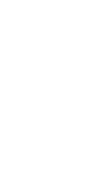
Figure 3.1 Factor model for two variables. Free parameters are indicated by x, y and z. Causal paths are shown as single headed arrows and correlational paths are shown as double-headed arrows.
Syntax:
#define <name> <number>
Various commands and keywords used in Mx scripts search for a number. During this search, if Mx encounters a letter it will read the word and check the dictionary for matching #define'd words. If the word is found, the appropriate number is substituted. If it hasn't, a warning will be printed and the search for a number or a #define'd variable will continue. Care is needed with spelling!
In multivariate modeling it is quite common that the same matrix dimensions are used in many different parts of a script. For example, in an oblique factor analysis, with 10 observed variables and 2 factors, the dimensions of the matrices needed to define the model are dictated by these numbers. If matrix L contains the loadings, P the correlations between the loadings, and matrix E the residuals, we would require L to be of order 10�2, P to be 2�2 and E to be of order 10�10. We might specify this in Mx with a script of the form
Title - factor analysis
Data NInput=10 NObservations=100
CMatrix File=mydata.cov
Matrices
A Full 10 2 Free
P Stan 2 2 Free
E Diag 10 10 Free
Covariance A*P*A' + E /
Start .5 all
End
However, this script could be made more general with a couple of #define statements:
#define factors 2
#define vars 10
Title - factor analysis
Data NInput=vars NObservations=100
CMatrix File=mydata.cov
Matrices
A Full vars factors Free
P Stan factors factors Free
E Diag vars vars Free
Covariance A*P*A' + E /
Start .5 all
End
Gain is small in this simple model - we change two numbers to change the number of factors and number of observed variables, instead of seven. With more complex models, the use of #define can make scripts much simpler and more versatile.
Syntax:
Begin Matrices; or Matrices= {Group <n>}
<matrix name> <type> <r> <c> {Free/ Unique}
....
End Matrices;
Matrices must be declared after reading any data for the group, and before assigning values or parameters to matrix elements. All declared matrices initially have zero for each 'modifiable' element. By default, all matrix elements are fixed. If the keyword Free appears, each modifiable element has a free parameter specified, starting at the highest parameter number yet specified below 10,000. If the keyword Unique is present parameters are numbered from 10,000 onwards. Unique helps to keep parameters from accidentally being constrained with subsequent specify statements. See page ? for more details on declaring matrices.
Syntax:
Begin Algebra;
<matrix name> = {funct} <matrix name> {operator <matrix name> };
...
End Algebra;
Algebra sections provide a simple way to evaluate matrix algebra expressions, as shown in Appendix C.
In many cases breaking up a complicated matrix algebra expression into smaller parts can improve readability or efficiency or both. For example, the matrix formula (I-A)~*S*(I-A)~' will find the inverse of twice. When matrix A is small the loss of efficiency will be negligible - the extra time taken to re-program will be greater than any gained in execution time. For large A, the component (I-A)-1 can be computed as an intermediate step so that the cpu-intensive matrix inversion is only carried out once and we have a compact and readable script. Algebra may be thought of as a special form o f matrix declaration. Each matrix that appears on the left hand side of the = sign is newly defined in this group (it must not have been previously defined). Note that matrix B, defined in the first line of algebra, may be used in subsequent lines.
Begin Matrices;
A Full 10 10
S Symm 10 10
I Iden 10 10
End Matrices;
Begin Algebra;
B = (I-A)~ ;
C = B*S*B' ;
End Algebra;
Every group has to begin with a Title line and a Group-type command. In a data group, these statements may be followed by reading of data. These commands are described in this section.
The title line is purely for the user's reference, it is printed when Mx prints the parameter specifications and the parameter estimates for a group. It is most useful when there are multiple groups. The title line is recognized by its location (the beginning of a group) rather than by a keyword at the start of a line.
Syntax:
Data/Calculation/Constraint {NGroups=n NInput_vars=n NObservations=n}
where Calculation defines a calculation group and Constraint a constraint group, the default being a Data group
Every group must have a data line. It has a number of parameters to indicate
The parameters may be specified in any order, and are summarized in Table 3.2. Note that Data groups must have NInput_vars and NObservations keywords. Constraint groups only require NInput_vars, and Calculation groups need no parameters except NGroups if it is the first group.
Table 3.2 Parameters of the group-type line in Mx input files.
| Parameter | Function | Required for group(s) |
| Data
Calculation Constraint NGroups NInput_vars Nobservations Nmodel |
Specifies a data group
Specifies a calculation group Specifies a constraint group Number of groups Number of input variables Number of observations Number of models |
Data
Calculation Constraint First group Data, constraint Data Weighted likelihood* |
* required for fitting mixture models only, see section 4.3 on page 68
Covariance and Correlation Matrices
Syntax:
CMatrix/KMatrix/PMatrix {Full} {File=filename}
In a data group, a covariance matrix may be read using the keyword CMatrix. By default, CMatrix expects to read the lower triangle of an NInput_vars x NInput_vars matrix, from the input file. If the keyword Full appears, then a full matrix will be read. The matrix is read in free format, that is, the numbers are expected to be separated by one or more blank spaces or carriage returns. If the keyword File appears, then Mx will read the data from a file. This latter method is generally to be preferred, since it keeps the data in one place. If the data are changed, it is not necessary to change every script that uses these data.
A FORTRAN format [in parentheses, e.g., (6F10.5)] for reading data must be the first line of a data file. If the first line just has * or (*) on it, the data are read in free format, i.e. numbers are separated by one or more spaces or new line characters.
Correlation matrices (KMatrix) and matrices of polychoric or polyserial correlations (PMatrix) are read in the same way as covariance matrices (CMatrix). Although the diagonal elements of these matrices are all 1.0, and could in principle be omitted, they are needed for Mx to read the file correctly. See page 119 for an example of special methods required for maximum likelihood analysis of correlation matrices.
Asymptotic Variances and Covariances
Syntax:
ACov/AVar/AInv {File=filename}
In order to use asymptotic weighted least squares or diagonally weighted least squares ( see p. 78) it is necessary to read a weight matrix. For compatibility with PRELIS (Jöreskog & Sörbom, 1986; 1993), Mx expects to receive a weight matrix multiplied by the number of observations. If the File= option is used, a PRELIS output file (created with the SA=filename or the SV=filename PRELIS commands) may be read. By default, Mx expects to receive an asymptotic weight matrix (ACov) whose size depends on (i) NInput_vars and (ii) whether a correlation matrix or covariance matrix has been input. If NInput_vars=k, then if CMatrix has been input, the number of rows in ACov is
An ACov line makes AWLS the default method of estimation for that group. If AWLS is requested on the Options line in a group without an ACov, and error will result. Similarly, DWLS is default if AVar is read.
Note that inverting the asymptotic covariance matrix can take an appreciable amount of time for large problems. Two facilities are available to combat this problem. First, the inverse of the matrix can be read instead. A simple Mx job could be used to invert and save the inverse, for example:
Commands to invert a 325x325 asymptotic weight matrix
Data Calculate NGroups=1
Matrices
P Symm 325 325
Compute P~ /
Matrix P File=weight.asy
Output MX%E=weight.inv
The inverse of the asymptotic matrix (AInv), saved in the file weight.inv could be used in place of the matrix itself, with a command of the form: AInv Full File=weight.inv . The Full keyword is essential here because Mx is agnostic about the symmetry of square matrices created in calculation groups. It is safer to assume that it is not symmetric to maintain consistency across applications. The second, alternative approach is to use the binary save feature described on page 98, which saves the whole job specifications.
A common error in reading data with CMatrix or ACov commands is to read them as full matrices when they are stored as symmetric, or vice versa. Mx attempts to be a bit smarter about this process. If a user forgets to put the Full keyword on the CMatrix line, but Mx detects an Mx-style data file that was saved in full format, it will read it as full instead.
Variable Length, Rectangular and Ordinal Files
Syntax:
VLength/Rectangular/Ordinal {File=filename} {Highest <numlist>}
Mx will read two types of raw data for multivariate normal maximum likelihood analysis.
Rectangular reads regular data, i.e. where every observation has the same number of input variables (NInput_vars on the Data line). Missing values may be specified with a . (dot) or another code (see Missing command on page 45). This is appropriate if there are relatively few missing data, or if missing data have been imputed.
VLength is a variable length record reader, which allows reading of raw data where there may be many missing values. The default (and mandatory) format for these data is free. A line with comments or * can be placed at the start of the file, but it will be ignored by Mx except for printing a warning and the line itself in the output file. The structure of a VLength file is:
For every case, the number of input variables must be on a line by itself. The identification codes must be integers that correspond to codes read by the ICodes command (see page 75). For example, a file might contain the following:
3
1 2 3 .33 .62 .95
2
2 3 1.4 -2.2
1
2 .37
This example reads 3 variables for the first observation, with identification codes 1 2 3, and data values .33 .62 and .95. The second observation has no data for variable 1, but supplies data for 2 and 3, while the third supplies data for variable 2 alone. By default, data of this type are fitted using the raw maximum likelihood fit function (see page 81).
It is quite simple to prepare VLength files with SAS or SPSS. However, caution should be exercised with SAS which uses a . for a missing value. Depending on the operating system under which you are running Mx, this dot may produce a file read error or be read as a zero. Here are a few lines of SAS code to output a VLength file from an array of two variables V{2}, either or both of which may be missing. The third and fourth lines need to be modified to declare the length of the array and to copy the required variables to the array into it. Certain applications may also need to change the format of the PUT statement that writes the data values.
DATA ONE; SET ZERO;
COUNT=0; NVAR=2; /* Number of variables in total !!Change!! */
ARRAY V{2} AT1 AT2; /* Set up array for variables !!Change!! */
DO I=1 TO NVAR; /* Count the non-missing observations */
IF V{I} NE . THEN DO; COUNT+1; END; END;
FILE MXVLFILE; /* Filename for future Mx input !!Change!! */
IF COUNT NE 0 THEN DO; /* Write observations if there are any */
PUT COUNT;
DO I=1 TO NVAR;
IF V{I} NE . THEN PUT I @@; /* Write the identifiers */
END; PUT;
DO I=1 TO NVAR;
IF V{I} NE . THEN PUT V{I} 13.6 +1 @@; /* Write the data values */
END; PUT;
END;
Note: format statements are not valid for either rectangular or VL files.
Similar to the rectangular command to read raw continuous data, the Ordinal file statement reads in ordinal data from a rectangular file. By default, a . (dot) character separated by spaces is recognized as a missing value, and this default may be changed by inserting a Missing command before the Ordinal statement. Ordinal data must be specified by integer categories, with the lowest category zero. The highest category in the ordinal data is automatically detected by Mx, but in some cases, especially multigroup analyses, it is necessary to override this default with a user specified value. The largest value in the data file must not exceed the corresponding value in the highest statement.
Syntax:
Missing=<code>
The missing command may be used to supply a character string other than . (dot) to be used for missing values, e.g. Missing=N/A. Note that Mx responds to the exact character string, and not the numerical value of that string. For example, if Missing=-1.0 has been specified, then neither -1 nor -1.00 would be recognized as missing.
Syntax:
Definition_variable <label>
...
Specification <matrix name> {element list} label {element list}
This feature allows 'multilevel' statistical analyses with VL or rectangular data files. Essentially, some variables may be assigned as definition variables which can then be used in constructing the model. Definition variables are automatically #define'd so that their names can be used in Specify statements. A matrix containing a definition variable changes for every case in the raw data file. See page 132 for an example that allows continuous moderators - effectively as many groups as there are cases in the data file. Labels should be provided for all variables before using the definition statement.
Syntax:
CTable <r> <c> {File=filename}
Mx will read contingency tables of order r by c. NInput_vars must be 2 for a group reading a contingency table. Both r and c must be greater than 1 but they do not have to be equal. A contingency table contains frequency data (or counts) such that each cell Cij indicates the number of observations falling in row category i and column category j. Normally, the frequencies supplied should be greater than or equal to zero.
If frequency data are read directly into the script, they need to start on a new line, following the CTable <r> <c> line.
Mx automatically handles incomplete ascertainment which the user can flag by supplying a negative number for cells that have not been ascertained (see example on p. 85). Instead of modeling means, the placement of thresholds on the underlying liability distribution is specified with the threshold statement, as shown on page 68.
The ordering of the categories should follow the natural numbering of the rows and columns, so that a table with a strong positive correlation between the variables would have large frequencies on the leading diagonal. Supplying a CTable changes the default fit function to the likelihood of observing the frequencies assuming a bivariate normal distribution of liability underlies the observed presence in a cell. See page 84 for details on fitting structural equation models to contingency table data.
Syntax:
Means {File=filename}
A vector of means, length NInput_vars may be read. When fitting models by maximum likelihood, a matrix formula for the predicted means may be provided. The joint likelihood of the means and the covariances is maximized, enabling tests of hypotheses about equality of means across variables or across groups.
Syntax:
Skewness/Kurtosis {File=filename}
Matrices of skewness and kurtosis may be read with these commands. These are provided for future developments in Mx that will allow model fitting to these types of data in addition to means and covariances. Currently there is no facility to use matrices read in this way. However, model fitting with higher moments could be done with user-defined fit functions (see page 85).
3.4 Label and Select Variables
Syntax:
Labels <list of labels>
Labels may be given for the observed data by issuing a Label command, before the Matrices command. These labels may be used to select variables, for example:
Data NGroups=1 NInput_vars=3 NObservations=171
CMatrix File=Cov.mat
Labels ALC1 ALC2 AGE
Select ALC2 ALC1 /
would read the lower triangle of a 3�3 covariance matrix from the file Cov.mat, and label the variables ALC1 ALC2 and AGE. The variables ALC2 and ALC1 are then selected for analysis, changing their original order. See also page 75 for details on labeling specified matrices.
Syntax:
Select <numlist or varlist> /
Variables may be selected for analysis using the Select command. The command may be used to reorder data or to pick a reduced number of variables for analysis. In either case, a ; or / must end the command. Select accepts integers which correspond to the order of the input variable. More conveniently, Select will operate on variable labels (see page 46). The command will work with raw data as supplied by the Rawdata or VLength commands (see pages 81 and 43).
Syntax:
Select If <label> {< = > ^< ^= ^>} value/
where ^ denotes not.
Select If may be used in conjunction with raw data (VL or Rectangular) to select a subset of the data for analysis. This feature is useful to eliminate outliers form a raw dataset, if a case number or id variable has been included. For example,
Rectangular File=mydata.rec
Labels casenum BMI skinfold1 skinfold2;
Select If casenum ^=253;
Select BMI skinfold1;
might be used to eliminate all cases where casenumber is 253.
Select with Variable Length Data
In combination with the VL or rectangular data, select changes the identification codes to consecutive integers starting at 1. For example, if the following Select line was read:
Select 3 4 2 /
a VLength record of the form:
4
1 2 3 4 .1 .2 .3 .4
would be changed to:
3
1 2 3 .3 .4 .2
thus the observation originally numbered 3 has become observation 1, observation numbered 4 has become observation 2, and observation numbered 2 has become observation 3. Select will automatically reduce the number of data vectors if there are no matches for a particular data vector and the codes in the Select line. The final number of vectors and observations used in the analysis is given in the output file.
Select cannot contain more numbers than the NInput_vars specified on the Data line. To do so would necessarily result in a singular correlation or covariance matrix. Likewise, the same variable cannot be selected twice.
3.5 Calculation and Constraint Groups
The use of calculation and constraint groups is very similar the use of groups that read data. All three types of group are fully command compatible with the exception of commands for reading data, which can be used by data groups alone.
The keyword Calc on the Group-type line indicates that the group is used for calculation. The calculated matrix formula from such a group is printed if the RSiduals command appears on the Options line. There are no restrictions on the type and dimensions of a matrix than can be produced with this command (other than memory limits). The result of the calculation may be used in later groups by using the =%En syntax when specifying a matrix, where n is the number of the calculation group. Note that there is a strict ordering within the input file; results cannot be taken from a calculation that has not yet occurred.
The Calc group provides a facility for printing out results of matrix operations. Any calculation group that is not followed by a constraint or data group is not calculated until the end of optimization, thus avoiding unnecessary waste of computer time.
Constraint groups may be used to impose nonlinear equality or inequality constraints among the parameters. Three special operators may be used to impose constraints between matrices. For example, suppose we wish to impose the constraint that x2+y2 =1 where x has parameter specification 1 and y has parameter specification 2. A constraint group to accomplish this might be:
Constrain parameters to ensure that x*x+y*y=1
Constraint_group
Begin Matrices;
A Full 2 1
I Iden 1 1
End Matrices;
Specify A 1 2 ! Put parameters 1 and 2 in to A
Constraint A'*A=I; !Inner product works out x*x+y*y
End Group;
If we wanted to impose the inequality constraint that x2+y2 >1 instead, then we would use the > symbol in the Constraint statement. Likewise, we could use < to specify a less than inequality. Only one <, > or = symbol may be used in a constraint statement. To specify range constraints such as .5< x2+y2 <1 it is possible to specify both constraints within the same constraint statement by concatenating them as two inequality constraints:
Constrain parameters to ensure that .5 < x*x+y*y <1
Constraint_group
Begin Matrices;
A Full 2 1
I Iden 1 1
H Full 1 1
End Matrices;
Matrix H .5
Specify A 1 2 ! put parameters 1 and 2 into A
Constraint (A'*A_
H) < (I_
A'*A); ! Inner product works out x*x+y*y
End Group;
Note that the constraints are made element by element. Using option RS we can see the results of imposing equality or inequality constraints.
Whenever Mx encounters a constraint group, it increases the number of degrees of freedom by the number of nonlinear constraints. This increase in the number of statistics is based on the assumption that each constraint identifies a parameter, which may not always be correct. The DF parameter on the Options line (see page 88) may be used to correct for failures of this assumption.
NPSOL, the optimization routine, treats constraints in an intelligent fashion; if it finds the derivatives of the constraint functions with respect to certain parameters to be zero, it does not calculate them during optimization. This means that if some of the specified constraint functions are always zero, little additional computational cost is incurred.
Care is needed to make sure that the constraints can be satisfied. If there is no feasible point for the constraints - for example, one of them always takes the value .5 - an IFAIL=3 error message is returned. One way to avoid such errors is to start optimization at a place where the constraints are satisfied.
4 Building Models with Matrices
What you will find in this chapter
All groups, be they constraint, calculation, or data, require at least one matrix in order to do anything. The next few sections describe the types of matrix that may be used, the operators that act on and between them, and ways of putting parameters and numbers into them.
4.1 Commands for Declaring Matrices
Syntax:
Begin Matrices {= Group <n>};
<matrix name> <type> <rows> <columns> {= <name> <group> / Free, Unique}
....
<matrix name> <type> <rows> <columns> {= <name> <group> / Free, Unique}
End Matrices;
where n is a previous group number
A group must have the 3-letter MAT command, followed by at least one matrix definition. As used throughout this manual, we recommend using non-abbreviated commands, such as Matrices.
Matrix names are restricted to one letter, from A to Z. The same letter may be used for different matrices in different groups. If a matrix is declared twice, a warning is printed and only the second declaration is kept.
Note that matrix definitions are group specific; for example, matrix A in group 1 does not have to be the same type or size as matrix A in group 2.
If the keyword = follows the Begin Matrices command, all matrices in that earlier group are automatically declared in the present group.
The type of a matrix may be one of the 12 forms described in Table 4.1, and its row and column dimensions are specified with integers. Once the type and size of a matrix has been defined, it cannot be changed.
Table 4.1 Matrix types that may be specified in Mx.
Note: number of free elements indicates the number of elements that can be altered by the user, where r is the number of rows and c the number of columns of the matrix.
Equating Matrices across Groups
Syntax:
<matrix name> <type> <r> <c> = <matrix name> <group number>
or
<matrix name> <type> <r> <c> = <special quantity> <group number>
Optionally, a matrix may be constrained to equal a matrix previously specified. For example, we could use the command
A Symm 3 3 = Y2
to equate matrix A in this group to matrix Y in group 2. In this example the current group must be number 3 or greater.
Several additional options allow constraints to other quantities found in previous groups, such as the observed or expected covariance matrix. For example, the command
B Full 2 2 = %E1
equates matrix B in this group to the expected matrix of group 1.
The special codes for constraining a matrix to equal those defined or computed in previous groups are shown in Table 4.2. These add to the flexibility of Mx.
Table 4.2 Syntax for constraining matrices to special quantities in previous groups.
| Symbol | Matrix Quantity | Dimensions |
| %On
%En %Mn %Pn %Fn |
Observed covariance (data) matrix | NIn�NIn
NIn�NIn 1�NIn NRn�NCn 1�1 |
Note: NIn is the number of input variables in group n following any selection; NR and NC are respectively the number of rows and columns in a contingency table, and may be requested only if group n has such a table.
It is especially important to note that none of the %E, %O, %M, %F and %P equalities may refer to groups that appear after the current group. When matrices are constrained to be equal in this fashion, the type and row � column dimensions of the earlier matrix are retained. If the two specifications do not agree, a warning is printed. Both the number of rows and the number of columns must be supplied for square matrices, but only the first is used to define the size of the matrix.
Equating Matrices to Computed Matrices
Syntax:
<matrix name> computed {<r> <c>} = <matrix name> <group number>
When matrices are declared with the Matrices command, a special type, computed, may be used to equate to a matrix which was defined within the algebra section of a previous group. Row and column dimensions are set to those of the previously calculated matrix, and may be omitted when declaring a matrix as computed.
Equating All Matrices across Groups
Syntax:
Begin Matrices = Group <number>;
The usual equating of matrices across groups is supplemented by a global facility. All the matrices defined in an earlier group are made available to the current group. This includes both matrices that are explicitly declared and those that are created in a Begin Algebra; ...End Algebra; section.
All changeable elements of matrices are initialized at zero and are fixed parameters, unless the Free keyword is used, in which case each changeable element is specified as a different free parameter. Examples of the results of using the keyword Free are shown in Table 4.3.
Table 4.3 Examples of use of the Matrices command to specify the dimensions of different matrix types. The keyword Free following each command makes each modifiable element in the matrix a separate free parameter, numbered in order as shown in the second column. In the third column, values of elements are shown, with ? representing a free parameter.
| Example command | Specification Matrix | Values |
| A Zero 2 3 Free | 0 0 0
0 0 0 |
0 0 0
0 0 0 |
| B Unit 2 3 Free | 0 0 0
0 0 0 |
1 1 1
1 1 1 |
| C Iden 3 3 Free | 0 0 0
0 0 0 0 0 0 |
1 0 0
0 1 0 0 0 1 |
| D Izero 2 5 Free | 0 0 0 0 0
0 0 0 0 0 |
1 0 0 0 0
0 1 0 0 0 |
| E Ziden 2 5 Free | 0 0 0 0 0
0 0 0 0 0 |
0 0 0 1 0
0 0 0 0 1 |
| F Diag 3 3 Free | 1 0 0
0 2 0 0 0 3 |
? 0 0
0 ? 0 0 0 ? |
| G Sdiag 3 3 Free | 0 0 0
1 0 0 2 3 0 |
0 0 0
? 0 0 ? ? 0 |
| H Stand 3 3 Free | 0 1 2
1 0 3 2 3 0 |
1 ? ?
? 1 ? ? ? 1 |
| I Symm 3 3 Free | 1 2 4
2 3 5 4 5 6 |
? ? ?
? ? ? ? ? ? |
| J Lower 3 3 Free | 1 0 0
2 3 0 4 5 6 |
? 0 0
? ? 0 ? ? ? |
| K Full 2 4 Free | 1 2 3 4
5 6 7 8 |
? ? ? ?
? ? ? ? |
More detail on specifying parameters in matrices is given in Sections 4.4 to 4.5.
Readers unfamiliar with matrix algebra may benefit from reading Appendix C, where examples and exercises are given. Readers familiar with matrix algebra may wish to examine Tables 4.4 and 4.5 for the variety of available operators and functions, and use this section for reference.
In ordinary algebra, operators such as + � and � have an order of evaluation established by convention. Multiply and divide are done before addition and subtraction. Multiply and divide are done in left-to-right order if they appear consecutively, as are addition and subtraction. We could say then, that � and � have priority 1, and + and have priority 2. Default priorities can be changed with the use of brackets ( ) which specify that operations inside the brackets are done first. For example, a+b�c=a+bc whereas (a+b)�c= ac+bc.
A similar hierarchy has been established for the matrix operators in Mx, and it too may be
revised by the use of brackets. Table 4.4 shows the matrix operators and their (default)
order of evaluation. Matrix algebra is subject to certain rules of conformability -
requirements about the size and shape of the matrices being multiplied etc. These rules are
listed in the right hand column of table 4, where ![]() denotes rows in matrix A and
denotes rows in matrix A and ![]() columns in matrix B. The number or rows of a matrix (
columns in matrix B. The number or rows of a matrix (![]() ) and the number of columns of
a matrix (
) and the number of columns of
a matrix (![]() ) are known as its dimensions. Two matrices A and B where rA=rB and cA=cB
are said to have the same dimensions.
) are known as its dimensions. Two matrices A and B where rA=rB and cA=cB
are said to have the same dimensions.
Table 4.4 Matrix operators available in Mx, together with their priority for evaluation.
See also Table 4.5 for matrix functions.
| Symbol | Name | Function | Example | Priority | Conformability |
| ~ | Inverse
Transpose |
Inversion
Transposition |
A~
A |
1
1 |
r=c
none |
| ^
* . @ & % + | _ |
Power
Star Dot Kron Quadratic Eldiv Plus Minus Bar Under |
Element powering
Multiplication Dot product Kronecker product Quadratic product Element division Addition Subtraction Horizontal adhesion Vertical adhesion |
A^B
A*B A.B A@B A&B A%B A+B AB A|B A_B |
2
3 3 3 3 3 4 4 4 4 |
none
cA=rB rA=rB and cA=cB none cA=rB=cB rA=rB and cA=cB rA=rB and cA=cB rA=rB and cA=cB rA=rB cA=cB |
A line has been drawn between the first two operators (Inverse & Transpose) and the rest because inverse and transpose are unary operators, that is, they operate on one matrix. The rest form a single new matrix from two matrices, and are thus binary operators. These operators are now described in detail.
Only square matrices may be inverted, but they may be either symmetric or non-symmetric. The inverse of matrix A is usually written A1 and implies that AA1 = A1 A = I where I is the identity matrix. To request an inverse with Mx, we use the symbol ~. If the inverse does not exist (possibly due to rounding errors), Mx will terminate with an error message. Some precautions can be taken to avoid this, such as supplying starting values that allow inversion, or putting boundary constraints on parameters to prevent their taking values that would lead to a singular matrix.
Any matrix may be transposed. The transpose of A is written A. The order of the matrix changes from r�c to c�r, as the rows become the columns and vice-versa.
All the elements of a matrix may be raised to a power using the ^ symbol. Essentially, this operator works the same way as the Kronecker product (see below), but elements of the first matrix are raised to the power of those in the second matrix instead of multiplied by them. It is possible to use negative powers and non-integer exponents to indicate reciprocal functions and roots of elements, but it is not possible to raise a negative number to a non-integer power. For example, the cube of every element of a matrix would be obtained by A^B if B was a 1�1 matrix with 3 as its only element.
For example, the matrix power A^B is

* or 'Star' is the ordinary form of matrix multiplication. The elements of A(m�n) and B(n�p) are combined to form the elements of matrix C(m�p) using the formula
![]() . Matrices multiplied in this way must be conformable for
multiplication. This means that the number of columns in the first matrix must equal the
number of rows in the second matrix.
. Matrices multiplied in this way must be conformable for
multiplication. This means that the number of columns in the first matrix must equal the
number of rows in the second matrix.
For example, the matrix product A*B

Dot is another type of matrix multiplication, which is done element by element. For two matrices to be multiplied in this way, they must have the same dimensions. Elements of the dot product are described by the formula Cij = Aij�Dij.
For example, the dot product A.D is

The right Kronecker product of two matrices A B is formed by multiplying each element of A by the matrix B. If A is of order (m�n) and B is of order (p�q), then the result will be of order mp�nq. There are no conformability criteria for this type of product. In Mx input files the symbol is denoted with the symbol @.
For example, the Kronecker product A B is

Many structural equation and other statistical models use quadratic products of the form ABA', and the quadratic operator is both a simple and efficient way to implement quadratics. Note that E can be any shape, but to be conformable for quadratic product the matrix B must be square and have the same number of columns as the matrix E.
For example, the quadratic product E&B
% does element by element division. For two matrices to be divided in this way, they must have the same dimensions. Elements of the result, C are described by the formula
Cij = Aij � Dij. If any element of D is zero, the corresponding cell in the result matrix is set to 1035.
For example, the division A%D is

Addition of matrices is performed element by element. For two matrices to be added, they must have the same dimensions. Elements of the sum, C are described by the formula
Cij = Aij + Dij.
For example, the sum A+D is

Subtraction of matrices is performed element by element. For one matrix to be subtracted from another, they must have the same dimensions. Elements of the difference, C are described by the formula Cij = Aij Dij.
For example, the difference AD is

Bar allows partitioning of matrices. Its operation is called horizontal adhesion because A|D is formed by sticking D onto the right hand side of A. For two matrices to be adhered in this way, they have to have the same number of rows. If A (m�n) and D (m�p) are adhered, the result C is of order (m�(n+p)).
For example, the operation A|D is

Underscore allows partitioning of matrices. Its operation is called vertical adhesion because A_D is formed by sticking D underneath A. For two matrices to be adhered in this way, they must have the same number of columns. If A (m�n) and D (p�n) are adhered, the result C is of order ((m+p)�n).
For example, the operation A_D is

A number of matrix functions, shown in Table 4.5, may be used in Mx. These are useful for in specialized applications involving user-defined fitting-functions (see p. 85).
Table 4.5 Matrix functions available in Mx.
Restrictions are on rows r and columns c of input argument.
| Keyword | Function | Restrictions | Result Dimensions |
| \tr( )
\det ( ) \sum( ) \prod( ) \max( ) \min( ) \abs( ) \cos( ) \cosh( ) \sin( ) \sinh( ) \tan( ) \tanh( ) \exp( ) \ln( ) \sqrt( ) \d2v( ) \v2d( ) \m2v( ) \vec( ) \vech( ) \stnd( ) \eval( ) \evec( ) \ival( ) \ivec( ) \mean() \cov() \pchi() \pdfnor() \mnor() \momnor() \allint() \aorder() \dorder() \sortr() \sortc() \part() |
Trace
Determinant Sum Product Maximum Minimum Absolute value Cosine Hyperbolic cosine Sin Hyperbolic sin Tan Hyperbolic tan Exponent (eA) Natural logarithm Square root Diagonal to Vector Vector to Diagonal Matrix to Vector Matrix to Vector* Lower triangle to Vector Standardize matrix Real eigenvalues Real eigenvectors Imaginary eigenvalues Imaginary eigenvectors Mean of columns Covariance of columns Probability of chi-squared Multivariate normal density Multivariate normal integral Moments of multivariate normal All integrals of multinormal Ascending sort order Descending sort order Row sort Column sort Extract part of matrix |
r=c
r=c None None None None None None None None None None None None None None None r=1 or c=1 None None None r=c r=c r=c r=c r=c None None r=1 and c=2 r=c+2 r=c+3 r�1 r�1 None None None |
1�1
1�1 1�1 1�1 1�1 1�1 r�c r�c r�c r�c r�c r�c r�c r�c r�c r�c min(r,c)�1 max(r,c)�max(r,c) rc�1 rc�1 rc�1 r�c r�c r�r r�1 r�r 1�c c�c 1�2 1�1 1�1 r�1 r�1 r�max(1,c-1) max(1,r-1)�c Variable� |
*vec: vectorizes by columns, in contrast to m2v, which vectorizes by rows.
� \part (A,B) takes two arguments. The elements of the 1�4 matrix B are used to define a rectangle within matrix A to be extracted.
Functions , called with syntax of the form \func(argument) differ from operators because they take an argument enclosed by parentheses (). This argument may be a single matrix name, or a complex matrix formula. The argument is evaluated before the function is applied, consistent with the rules for using brackets. Functions form a second set of unary operators (see page 54). Descriptions of these functions follow.
The trace of a matrix is the sum of the elements on the leading diagonal, i.e.
Properties of determinants, and ways of calculating them are discussed in Appendix C. This function is calculated for square matrices only.
The sum of a matrix is the sum of all its elements, i.e.,
The product function of a matrix yields the product of all its elements, i.e.,
The maximum function of a matrix yields a 1�1 matrix containing the maximum of all its elements.
The minimum function of a matrix yields a 1�1 matrix containing the minimum of all its elements.
The abs function replaces all matrix elements with their absolute value.
Trigonometric functions \cos( ), \sin( ) etc.
These functions replace all matrix elements with their appropriate trigonometric transformation, in radians.
Any matrix is a legal argument for this function which replaces each element Aij by eAij.
Any matrix is a legal argument for this function which replaces each element Aij by ln Aij. If an element is less than 1�10-30 then the result is ln (1�10 -31). Although error messages would be more normal in such a situation, this behavior can be helpful in optimization.
Any matrix is a legal argument for this function which replaces each element Aij by ![]() .
If an element is less than zero, a fatal error occurs.
.
If an element is less than zero, a fatal error occurs.
The leading diagonal of any matrix is placed into a column vector with min(RbC) rows, i.e. r or c, whichever is less. e.g.

Vector to Diagonal Matrix \v2d( )
A row or column vector is placed in the leading diagonal of a square matrix. e.g.

A matrix is placed in a column vector, by rows. Thus

A matrix is placed in a column vector, by columns. Thus

Note that it is more efficient to use \m2v(A) than \vec(A') and more efficient to use \vec(A) than \m2v(A'). Both functions work for matrices of any shape.
All the elements on the diagonal and below are placed into a vector, by columns. Thus


This operation converts a covariance matrix into a correlation matrix. Replacement of elements is made according to the formula:
The real parts of the eigenvalues of a square matrix are placed in a column vector, in ascending order of size, smallest first.
The real parts of the eigenvectors of a square matrix are placed in a square matrix, where column j contains the eigenvector corresponding to eigenvalue j, with eigenvalues sorted in ascending order of size, smallest first (j=1).
Imaginary Eigenvalues \ival( )
The imaginary parts of the eigenvalues of a square matrix are placed in a column vector, in ascending order of size, smallest first.
Imaginary Eigenvectors \ivec( )
The imaginary parts of the eigenvectors of a square matrix are placed in a square matrix, where column j contains the eigenvector corresponding to eigenvalue j, with eigenvalues sorted in ascending order of size, smallest first (j=1).
This function computes the means of the columns of a matrix.
This function computes the covariance matrix of the columns of a matrix. Thus if data are presented as one line per subject, with r rows for each of the c variables, the output would be of order c�c.
Probability of Chi-square \pchi(x)
Function \pchi computes the probability of a chi-squared with nu degrees of freedom. Its argument must be a 1x2 vector containing the chi-squared and degrees of freedom. It returns a 1x1 matrix. This can be useful when writing parameter estimates and fit statistics to a file.
Multivariate Normal Density \pdfnor(A)
The function \pdfnor computes the multivariate normal probability density function (pdf) given by the multivariate normal distribution. In the univariate case, this is the height of the normal curve. Matrix A, the argument of the function, is a nvar+2�nvar matrix, containing: (first row) a vector of observed scores xi; (second row) a vector of population means �i; and (rows 3 to nvar+2) the population covariance matrix . The pdf is
The matrix function \mnor will compute multiple integrals of the multivariate normal, up to dimension 10. Its input is structured so that for n dimensional integration, the matrix has n columns and n+4 rows. The first n rows define the covariance matrix, row n+1 defines the mean vector, the last three are used to define the type of truncation experienced by each variable. This is best described with an example. The script:
Test multivariate normal integral function
Data Calc NGroups=1
Matrices
A full 1 2 ! Upper limits
B full 1 2 ! Lower limits
T Full 1 2 ! Type of integral
R Stan 2 2 ! Covariance matrix
Z Full 1 2 ! Means
Compute \mnor((R_Z_A_B_T)) /
Matrix R .3
Matrix B 0 0
Matrix A 1 1
Matrix T 2 2
Option RSiduals
End
computes the integral of the bivariate normal distribution with correlation .3 from 0 to 1 in both dimensions. The type parameters (matrix T) are flags that indicate the type of truncation required:
where aj and bj are the elements of column j of matrices a and b.
Accuracy is set to six decimals by default. Lower precision may be set with Option Eps=<value> though it should be noted that this option will be treated globally, i.e., for all such integrals in a particular run.
Moments of the Truncated Multinormal \momnor( )
The matrix function \momnor will compute moments of the truncated multinormal distribution. Currently, it will work only with 'tails' of the distribution, though selection may be absent for some variables. Here is a bivariate example:
Test moments of truncated normal function
Data Calc NGroups=1
Matrices
R Symm 2 2 !covariance matrix
M Full 1 2 !means
T Full 1 2 !thresholds
S Full 1 2 !selection vector
N Full 1 2 !# of abscissae
Compute \momnor((R_M_T_S_N)) /
Matrix R 1 .5 1
Matrix M 0 0
Matrix T 1.282 1.282
Matrix S 1 1
Matrix N 16 16
Option RSiduals
End
This script requests the covariances and means of individuals selected above the threshold 1.282 in a N(0,1) bivariate normal distribution. It returns the covariance matrix in the first n rows, and the means in row n+1.
Note: this function can give incorrect results when the number of abscissae is small, or the thresholds are extreme (more than 3 standard deviations from the mean). CPU time will go up with the number of abscissae, but 64 is the maximum (and it goes in jumps 16 20 24 32 48 64, along with some smaller jumps below that). Mx automatically assigns the number of abscissae to: i) 16 if you enter 0 or less, ii) 64 if you enter 64 or more, and iii) the next lowest value if you happen to chose an intermediate value (e.g. it will pick 24 if you enter 30).
All Intervals of the Multivariate Normal Distribution \allint()
It is often necessary to compute the probabilities of all the cells of a multivariate normal that has been sliced by a varying number of thresholds in each dimension. These thresholds are more formally called hyperplanes. While it is possible to use the \mnor function to achieve this goal, it can be more efficient and more convenient to use the \allint function. The argument to the \allint function must be a matrix with as many columns as there are variables, and with as many rows as the number of columns plus 2 plus the maximum number of thresholds to be evaluated. The general form is \allint(R_X_T_A) where R is the m � m covariance matrix of m variables, X is the mean vector, T is a row vector whose elements ti specify the number of thresholds in dimension i, and A contains the thresholds and is of order (max(ti) � m).
\Allint returns the proportions in all the cells, cycling from lowest to highest with the last variable in R changing most slowly. For example, the following script:
#NGroups 1
#define nvar 2 ! number of variables
#define maxthresh 3 ! maximum number of thresholds
Test of allint function
Calculation
Begin Matrices;
A symm nvar nvar
N full 1 nvar
X full 1 nvar
T full maxthresh nvar
End Matrices;
Matrix A 1 0 1 ! identity matrix here
Matrix X 0 0 ! zero means
Matrix N 2 3 ! first dimension has 2 thresholds (3 categories), second has 3
Matrix T
-1.282 -2.323 ! thresholds are -1.282 and 0 for first dimension,
0 0 ! and are -2.323, 0 and 1.282 for second dimension
10 1.282 !
Begin Algebra;
C = \allint(A_X_N_T) ;
End Algebra;
End Group
will return:
MATRIX C
This is a computed FULL matrix of order 1 by 12
[=\ALLINT(A_X_N_T)]
1 2 3 4 5 6 7 8 9
1 0.0010 0.0490 0.0400 0.0100 0.0040 0.1960 0.1601 0.0400 0.0050
10 11 12
1 0.2450 0.2000 0.0500
containing the desired probabilities.
This function gets the ascending order of a column vector. For example, \aorder(A) with

This function gets the descending order of a column vector. For example, \dorder(A) with

Used to sort a column vector or matrix by rows. If a vector, the vector elements themselves are sorted. If a matrix, the first column is taken to be the sort order - and must contain a permutation of the integers 1 to the number of rows, as might be extracted using, e.g., \aorder() above.
This function works the same way as \sortr() but by columns.
This function extracts a rectangular sub-matrix of matrix A (formerly this was possible only by pre- & post-multiplying by elementary matrices). One has to be very careful to initialize matrix B before this statement is given, because the result dimensions are needed to check syntax. To pre-initialize B you would use the following job structure
Title
Calculation NGroups=1
Begin Matrices;
A Symm 3 3
B Full 4 1
End Matrices; ! <- End matrix definitions with this statement
Matrix A
1
2 3
4 5 6
Matrix B 2 1 3 3
Compute \part(A,B) / ! <- Compute statement *after* matrix statement
Option RSiduals
End
The format for matrix B is row, column, row, column so in this example the rectangle from 2,1 (row 2, column 1) to 3,3 will be extracted, giving
2 3 5
4 5 6
Note that the elements of B may define any two opposite corners of a submatrix of A. To some extent, the \part() function is binary, but we prefer to list it with the other matrix functions.
A matrix formula is a sequence of matrix names and matrix operators terminated by a semi-colon. For example
A*B + \m2v(C);
Syntax:
Covariances/Compute formula;
The covariance command uses the matrices specified following the Matrices command and special symbols to perform operations or functions on or between them. A Covariance statement may contain a single matrix and no operations, or it could be very complex. The command may extend over several lines and must end in a ; or /. Compute is the recommended keyword for calculation groups, to make reading scripts easier for humans.
The primary method of carrying out matrix algebra is within an algebra section (see page 40). Matrices that appear on the left hand side should not already exist in that group.
Syntax:
Means A formula;
The Means command operates in the same way as the Covariance command. It exists to facilitate the modeling of means. All the matrix operators and functions (Section 4.2) may be used just as when specifying a model for covariances. A ; or / must end the command. Currently, Mx will do nothing with models for means when applying the functions LS, GLS, AWLS, DWLS. Only the ML, US and RM fit functions make use of models for means.
Syntax:
Threshold A formula;
The Threshold command operates in the same way as the Means to specify thresholds. It enables modeling of thresholds when fitting to contingency table data. All the matrix operators and functions (Section 4.2) may be used just as when specifying a model for covariances. A ;or / must end the command. Threshold cannot be used with any fit function other than contingency table ML, which is used when CTable data have been supplied (see chapter 5).
Special restrictions apply to the dimensions of the matrix calculated in the Threshold command. The result must have 2 rows and must have at least d columns where d=max ((r-1),(c-1)), in other words, at least one less than the number of rows or the number of columns in the contingency table, whichever is the greater. The first (r-1) elements of the first row of the matrix will contain the thresholds that separate the rows. The first (c-1) elements of the second row of the matrix will contain the thresholds that separate the columns. These elements are unstandardized row and threshold estimates, which may be standardized by dividing by the square root of the product of the two diagonal elements of the expected covariance matrix calculated by the Covariance or Constraint statement. Use of unstandardized thresholds allows the testing of models that predict differences in variance between groups, but have equal thresholds.
The user should take care to supply starting values for thresholds that increase from left to right in both rows of the matrix calculated by the Threshold command. Ideal starting values are those that, when standardized, mark the z-scores on the normal distribution corresponding to the cumulative frequencies of the normal distribution of the row totals (first row of the calculated matrix) or the column totals (second row of the calculated matrix). For example, if the following contingency table was supplied as data:
CTable 3 2
20 180 40
360 20 180
then appropriate starting values for 2 row thresholds would be -.67 and +.67 (z-scores corresponding to the lower 25% and 75% of the normal distribution), and -1.28 would be appropriate for the starting value of the column threshold (z-score corresponding to the lower 10% of the normal distribution). Therefore if the threshold model was simply T, we would declare
T Full 2 2
and use
Matrix T -.67 .67 -1.28 0
to initialize it.
Syntax:
Weight <formula> ;
where formula is a legal matrix algebra formula
The fundamental assumption of fitting a model to a population is that there is only one model. However, the population may consist of a mixture of groups which differ in the parameters or the entire structure of the model. In Mx, the weight command, coupled with the Nmodel parameter, allow analysis of such mixtures when the raw data are available. NModel controls the number of models supposed to exist in the population. The predicted means and covariances are simply vertically stacked in the usual matrix expression for the means and covariances. For example, if three variables were being studied with one model, the predicted mean vector would be of order (1�3) and the predicted covariance matrix would be (3�3). If two models are being used, the predicted mean vector should be (2�3) and the predicted covariance matrix (6�3). Mx checks that the size of the predicted covariance and mean vectors agree with the NModel and NInput (including any changes made with Select/Definition statements). Weight allows modeling of the likelihood that a particular observed vector is a member of a particular model class. The weight matrix expression should evaluate to a vector of order (NModel�1). The log-likelihood for a particular vector then becomes:
Often, the weights used will reflect simple proportions, and usually wi = 1. (see page 134 for an example). Sometimes, covariates may be used to compute the weight applied to a particular model. An example of such weighting is quantitative trait loci analysis where the probability that a pair of siblings have 0, 1 or 2 alleles in common at a particular place on the genome can be used to weight their likelihood under three models (Eaves et al., 1996).
Syntax:
Freq <formula> ;
where formula is a legal matrix algebra formula
For maximum likelihood analysis of raw continuous data, it is possible to enter a formula for the frequency of the individual observations. For a constant frequency that does not change across the individual cases, this formula could be a scalar (1x1) matrix with the weight in it. More commonly it is desired that the frequency changes across the observations, in which case the use of definition variables to assign variables read in as data to the elements of matrices may be used.
4.4 Putting Numbers in Matrices
This section describes three methods of entering numbers into matrices (see Section 4.5 for how to specify elements of matrices to be free, fixed or constrained parameters). In Section 3.1, we saw how matrices could be declared as one of 11 types, such as identity, symmetric, diagonal or full (see Table 4.1), and how their dimensions (rows, r and columns, c) were specified. On inspection of the table, we see that types Zero, Identity Identity|Zero and Zero|Identity (IZ) have no free elements at all. For example, there is nothing more to know about an IZ matrix which has 2 rows and 4 columns. It looks like this:
All six remaining matrix types have modifiable elements which may be altered with the commands Matrix, Start or Value. The number of modifiable elements varies according to:
All modifiable elements of a matrix are initialized at zero. The order of elements in a matrix is left to right, by rows. For example, a symmetric (3�3) matrix would be read as:
1
2 3
4 5 6
See Table 4.3 for more examples on the patterning of matrices.
Syntax:
Matrix <matrix name> {File=filename} <numlist>
where <numlist> is a free format list of numbers.
Note that different syntax is required in multiple fit mode:
Matrix <group number> <matrix name> {File=filename} <numlist>
The Matrix command supplies a list of values for the modifiable elements of a matrix. The list length required varies according to matrix type, and size as described at the start of this Section, on page 70. For example, suppose we specify a diagonal matrix A with 3 rows and 3 columns. The fourth column in Table 4.1 shows that the number of free elements is equal to r for diagonal elements, so we supply r elements. The command lines
Matrix A .3 5 9
or, equivalently
Matrix-I-would-like-to-change-is A
0.3D+00 5 9.00000000
would result in matrix A as:

Matrix will read its elements from a file with a FORTRAN format on the first line. Such files may have been produced by an earlier run of Mx, or by another program. LISREL matrix output files (produced by commands such as gamma=filename on the LISREL OU line) are fully compatible. The files must contain at least as many numbers as required to fill the changeable elements of the matrix specified (see page 70).
Mx always expects a format, so a * should be supplied for matrices in free format (numbers separated by blanks and carriage returns).
Syntax:
Start/Value <value> <element list>/ All
where <element list> consists of matrix elements (e.g. A 1 2 3) and may include the TO keyword
In a large matrix, it is not convenient to provide a value for all the elements of a matrix, when only a few need to be modified. Under these circumstances, it is easier to explicitly change elements by name. Elements may be referred to by up to three subscripts, according to the syntax
A {<group>} <row> <col>
If the matrix you wish to refer to is in the current group, the group number may be omitted. The numbers <group> <row> <col> may be separated by any number of non-numeric or blank characters, so that, for example, to put .5 in row 2 column 3 of group 1's A matrix, you could enter:
Value.5 A 1 2 3
will work the same as
Value.5 A(1,2,3)
N.B. It is only possible to modify matrices declared in the current or previous groups.
Value and Start recognize #define'd variables (see page 39). For example. We could have the statements
#define first 1
#define rowsinA 6
#define colsinA 10
at the top of the script, and then
Value 1.5 A first 1 1 to A first rowsinA colsinA
would set 1.5 to all the fixed (non-free) elements of A, from A 1 1 to A 6 10.
The difference between Start and Value lies in their treatment of elements when the keywords ALL or TO are used ( is a synonym for TO). With the keyword ALL, Start assigns a starting value to every free parameter specified at that point in the input file. Value does the opposite -- it assigns its value to every fixed matrix element specified up to that point. Although Start does the same thing if the TO keyword is specified, i.e. only apply its value to free parameters, Value behaves differently. It will assign a value to all elements in the same specified range, free parameter or fixed.
The TO keyword should be used only to specify a range of matrix elements within the same matrix.
4.5 Putting Parameters in Matrices
Parallel to the placement of numbers in matrices described in Section 4.4, there are facilities for putting parameters in matrices. Note also that all modifiable elements of a matrix can be specified as different free parameters using the keyword Free after the matrix is specified (see Section 4.1), and that building models with this in mind can be much faster and more flexible (see Chapter 1).
Syntax:
Pattern <matrix name> {File=filename} <numlist>
where <numlist> is a list of 1's and 0's.
Note that different syntax is required in multiple fit mode:
Pattern <group number> <matrix name> {File=filename} <numlist>
The Pattern command is a simple method that has the same syntax as the LISREL command on which it was based. Following the Pattern command, the user must provide the correct number (see Matrix command page 70) of 1's and 0's for that matrix. A 1 (or any non-zero value) indicates that the element is a free parameter (which may be constrained to equal another free parameter - see the Equate command on page 73), and a 0 indicates that the element is fixed.
Syntax:
Fix/Free <value> <element list>
where <element list> is a list of modifiable matrix elements
The Fix and Free commands operate directly on specific matrix elements or sets of matrix elements. Fix makes a parameter fixed (if it was Free before) and Free makes an element a free parameter to be estimated. Matrix elements are referred to by group, row and column as described in page 71. The keywords TO and ALL may be used to specify ranges of matrix elements to be fixed or freed. See page 98 for alternative methods to fix parameters.
For example, suppose in group 1, matrix A was defined as symmetric, with 4 rows and columns. Initially it would be patterned with zeroes throughout. The command
Free a 1 2 1 - a 1 4 3
would give the following pattern:

Fix A 1 4 2
the parameter specification would become:

Syntax:
Equate <matrix> {<gp>} <r> <c> <matrix> {<gp>} <r> <c> ...} }
In order to constrain matrix elements to equal one another, the Equate command may be used. Its primary purpose is to specify equality constraints among parameters, but it can be used to copy a numeric value from one matrix element to another. There is a big conceptual difference between the first element specified in a list and the others. The fixed or free status of the first element is given to the remaining elements in the list, be they fixed or free. If the first element is a free parameter, the same parameter is copied to the other elements. If the first element is fixed, then a warning message is printed, to the effect that all other elements will be fixed. The value in the first element is then passed to the other elements in the list. The Equate command may be used within matrices, or across matrices in the same group, or across matrices in different groups. Note that it is not possible to use Equate to make an immovable element (such as an element of a matrix specified as type ID, or an off-diagonal element of a diagonal matrix) into a free parameter.
For example, given matrices specified in group 1 as follows:
Begin Matrices;
A Symm 3 3 Free
B Full 2 4
I Identity 6 6
End Matrices;
the following Equate statements are legal:
Equate A 1 1 B(2,2) B 1 4
Equate B 2 1 A 1 2 3
Equate BANANA 2 2 APPLE 1 1 1
However, the following are illegal:
Equate A 1 1 I 2 2 (a)
Equate I 5 5 B 1 1 (b)
Equate A 1 2 C 1 1 (c)
Equate A 4 4 B 1 1 (d)
Equate A 2 2 G 4 1 1 (e)
They fail because: I is an identity matrix (a & b), C has not been specified (c), A does not have 4 rows and columns (d), and it is not possible to refer to an element of a matrix in a later group (e).
For large models with many constraints it is often more efficient to use the Specification command, or to seek repetitive structures in the model matrices and use partitioned matrices (see Chapter 1), or both. The kronecker product can be particularly useful when specifying repetitive partitioned matrix structures.
Syntax:
Specification <matrix name> a { b {c}}
where a, b and c are not necessarily distinct integers.
Note that different syntax is required in multiple fit mode:
Specification <group number> <matrix name> a { b {c}}
Following the Specification command, the user supplies a list of numbers that varies in length according to the dimensions and type of the matrix (see Section 4.4). If a zero is supplied, it indicates that the element is to be fixed. Non-zero elements refer to free parameters, and the same number refers to the same parameter. For example, the command
Specification A
1 2 3 0 0 0
0 0 0 3 2 1
would be equivalent to the statements
Pattern A
1 1 1 0 0 0
0 0 0 1 1 1
Equate A 1 1 A 2 6
Equate A 1 2 A 2 5
Equate A 1 3 A 2 4
The second method becomes tedious and error-prone in large models.
Note that the Specification and Pattern commands cannot be mixed in the same Mx job. This is for safety, because the opportunities for user error are too large.
Syntax:
Bound low high <parlist> / ALL
where <parlist> is a list of matrix elements or a list of parameter Specification numbers.
By default, parameters to be estimated are constrained to lie between -10000 and +10000. These limits can be increased or decreased with the Bound command. Boundaries may be supplied more than once for any parameter, but only the last Bound statement referring to a particular element is used. For example the statements
Boundary -1 1 all
Boundary .3 5 a 1 4 6 a 1 5 6
would change the limits for all parameters to -1 and +1, except those (if any) in elements A 1 4 6 and A 1 5 6. The TO syntax may be used to specify ranges within matrices, so that
Boundary 0 1 X 1 2 to X 1 6
would make parameters in all elements between X 1 2 and X 1 6 lie take values between zero and one. If the Specification command has been used to specify parameters in matrices, then it may be easier to refer to parameters with these numbers in a Bound command. Thus
Specification A
0 2 4 6
2 0 6 7
Boundary 0 10 2 4
would be permitted as a method of bounding parameters 2 and 4 to lie between zero and ten.
Linear and Non-Linear Inequality Constraints
See page 48 on the use of constraint groups to implement inequality constraints.
4.6 Label Matrices and Select Variables
Syntax:
Labels Row/Column <matrixname> <label-list>
After matrices have been declared, whether within a Matrices or Algebra section, labels may be given for the row or column (or both) of any matrix that has free elements. Matrices without free elements (Zero, Identity, Identity|Zero, and Zero|Identity and Unit) are never displayed so labels provided for these matrices will not appear on the output. The label-list contains labels separated by blanks or carriage returns. Labels must not begin with a number and may be up to 8 characters long. More characters can be read, but Mx only regards the first eight as significant, and will only print the first eight on the output.
Labels may be given for the observed data by issuing a Label command before the matrices command, as described in Section 4.6.
Syntax:
ICodes <numlist>
where <numlist> is a number list of length NInput_vars.
The ICodes command may be used in conjunction with the VL or rectangular data to specify a non-standard structure of the expected covariance matrix. It may be thought of as a select command which operates on the predicted covariance matrix and predicted mean vector. By default, the identification codes for the covariance matrix are 1 2 3 4... For example, if NInput_vars=3 then by default the expected covariance matrix has a structure like this:

1
1 .1
1
2 .2
1
3 .3
2
1 2 .1 .2
2
1 3 .1 .3
2
2 3 .2 .3
3
1 2 3 .1 .2 .3
and any of these could be reordered. For example, if the following VLength data were input:
2
3 1 .9 .4
Mx would generate a covariance matrix of the form

The ICodes command allows the default order 1 2 3... to change, making an infinite variety of input data vectors readable. The repetition of a number is most useful for pedigrees of variable structure, for example, if the model generates the covariance between two parents and two children, data that come from families with more than two children may be handled. In this case, the ICodes command would be:
ICodes 1 2 3 3
And thus the covariance matrix looks like this:

3
3 3 3 .2 .4 .6
then Mx would create the following covariance matrix for this data structure:

5 Options for Fit Functions andOutput
What you will find in this chapter
Syntax:
Options <multiple> <fitfunc> <statout> <optimpar> <write> End \
where <multiple> starts multiple fit mode, <fitfunc> specifies the fit function, <statout> requests statistical output, <optimpar> requests optimization parameters, and <write> specifies the filenames to write matrices to files
The Option lines of Mx allow the specification of a wide variety of keywords and parameters to control the type of fit function used, the amount of output requested, file names for result matrices, and many others. The Option command does not signify the end of a group, so several Option lines may be given within any group. Option commands should follow Model or Covariance statements, and should not be followed by Bound commands. To end a group, the End Group; command is used, for example,
Option Mxa=Afile.out
Option RSiduals NAG=30
End Group;
5.2 Fit Functions: Defaults and Alternatives
The fit function for a group is automatically set according to the type of data that are read. For example, if covariance matrices alone are read, the default is maximum likelihood. Table 5.1 shows the default fit functions selected by Mx for a given data input. Note that the method may change between groups. If a function that does not asymptote to 2 (e.g. RU or RM) is used in any group, then no 2 probability is given at the end of optimization. In general, the default fit function is appropriate for the data supplied. Mx does not provide for altering the input data from one type to another (e.g. converting a covariance matrix to a correlation matrix). However, it is a simple task to write a separate Mx script to make this conversion.
Table 5.1 Default fit functions according to the type of data that have been read.
| Input data | Default fit function |
| CMatrix, KMatrix or PMatrix
CMatrix, KMatrix or PMatrix with ACov CMatrix, KMatrix or PMatrix with AVar |
ML
AWLS DWLS RM MLN |
CMatrix - covariance matrix; KMatrix/PMatrix - correlation matrix; ACov - asymptotic covariance matrix; AVar - asymptotic variance matrix; Radiata - Raw data; VLength - variable length data; Rectangular - rectangular file; CTable - contingency table;
ML - maximum likelihood; AWLS - asymptotic weighted least squares; DWLS - diagonal weighted least squares; RM raw maximum likelihood; MLN - maximum likelihood assuming bivariate normal liability.
There are several good introductions to the properties of different fit functions (e.g Jöreskog & Sörbom, 1989; Bentler, 1989). Controversy exists about the relative merits of the different methods in the face of assumption violations (see Kaplan, 1990), and it seems wise for the user to treat this information in the same way as a white wine from the Loire (drink youngest available). Currently, maximum likelihood (ML) is showing robustness in the face of violations of the assumptions of multivariate normality. Asymptotic weighted least squares (AWLS) generally performs better in the presence of kurtosis, but can be at least as badly affected by skewness as ML. See however, simulation work by Rigdon and Ferguson (1991) for problems with tetrachoric correlations.
In the following sections, the calculation of the fit functions is described, where S is the observed covariance matrix, is the expected covariance matrix, tr(A) indicates the trace of and |A| indicates the determinant of matrix A. S and are of order p and df is one less than the sample size used to calculate S.
The unweighted least squares fit function is calculated by the formula:
When model fitting to covariance matrices, the maximum likelihood fit function is
and this is modified when both a mean vector x and a model for the means � (see page 67) are supplied, this function is augmented to become
Generalized least squares is based on the principles of Aitken (1934-35); see Browne (1974)
Asymptotic weighted least squares AWLS
Asymptotic weighted least squares follows from work by Browne (1982, 1984) and others. Effectively, the variance covariance matrix of the observed summary statistics is used as a weight matrix W. Formally the fit function is
An alternative approach to maintaining a diagonal of ones would be to standardize the expected covariance matrix before calculating the AWLS fit function. Mx does this if the keyword Standardize appears on the Options line. Some care with starting values is needed here, because the solution for a model standardized in this way is necessarily not unique. A third approach would be to use a nonlinear constraint group (see Section 3.5) that constrains the diagonal elements to equal unity.
Diagonally weighted least squares DWLS
Diagonally weighted least squares is a simplified form of AWLS for use with large problems where the AWLS matrix becomes unmanageably large. It is a compromise with less statistical validity than AWLS and should be used with caution. Select does not work with DWLS to discourage its use. The fit function for DWLS is simply:
Least Squares - Maximum Likelihood LSML
This fit function starts with unweighted least squares, and takes parameter estimates from the solution as starting values for maximum likelihood estimation. This method is useful to avoid having to specify starting values that generate a positive definite covariance matrix. Its disadvantage is that it consumes more computer time than would supplying appropriate start values and using ML alone. Though more robust to bad starting values, it is not infallible; optimization is not (yet) an exact science.
Maximum Likelihood Analysis of Raw Continuous Data
When we have a sample of complete multinormal data, the summary statistics of means and covariance matrices are sufficient statistics to obtain maximum likelihood estimates of parameters (see the keyword ML above). It is common practice to remove from analysis any subject that has missing data. However, there are occasions when missing data result in the omission of a significant amount of data from analysis. If the number of types of missing data is small, for example, if there are really two sub-populations, one that has data on 6 tests, and one that lacks data on the fourth test, then covariance matrices could be computed separately for the two populations and models fitted separately to the different groups. Mx is flexible, allowing different groups to have different numbers of input variables.
This multi-group approach breaks down if the number of sub-populations is large and the sample size for each group is too small to estimate a positive definite observed covariance matrix (this happens if the number of variables exceeds the number of subjects). For this reason, a number of methods of handling incomplete data are provided in Mx. RM (raw maximum likelihood) is really an extension of the multigroup method described above, but calculates twice the negative log-likelihood of the data for each observation. The procedure follows the theory described by Lange et al., (1976). If there are k observed variables in the set, the normal probability density function of an observed vector xi is
Maximum Likelihood Analysis of Raw Ordinal Data
Data analysis proceeds by maximizing the likelihood under a multivariate normal distribution model. In order for this to take place, it is necessary to supply both a matrix formula for the covariances and a matrix formula for the thresholds. The covariance formula must result in a matrix which is square, symmetric (8) and has the same order as the number of variables read in from the Ordinal file. The threshold statement must yield a matrix which has the same number of columns as the number of variables being analyzed. The number of rows of this matrix must match the maximum category of all of the variables in the data file, or if the highest statement is used, the largest value in the argument to this command. This maximum category of all is known as maxcat.
For a vector of observed ordinal responses y = (y0, y1, ... ym), the likelihood is computed by the expected proportion in the corresponding cell of the multivariate normal distribution. Let the highest category of variable j be denoted by hj, and let tij denote the jth threshold of variable i. The expected proportion in the categories of y is computed as:
To illustrate in a trivariate case, the two vectors of observations
0 2 1
and
. . 1
would have likelihoods computed as:
An especially important feature of the maximum likelihood raw data approach is that it provides a natural method of handling missing data that are so common in longitudinal and multivariate studies. In theory, data that are missing completely at random (MCAR) or missing at random (MAR) are correctly handled by this procedure and will provide unbiased maximum likelihood estimates as long as the assumptions of the multivariate normal hold (Little & Rubin, 1987). This is entirely analogous to the continuous case. Failure to include cases that contain missing observations can lead to bias in parameter estimates. Elimination of such cases will almost always lead to larger confidence intervals on all parameters.
A further advantage of the raw data approach is that it provides a natural way to exploit moderator variables, using the definition variable methods described on pages 33 and 132. At this time it is only possible to model binary variables via path diagrams in the graphical interface, because the GUI always generates a script with a single vector of means, and not a matrix of thresholds. In the case of binary variables, the method will work from diagrams because Mx treats the mean and threshold statements equivalently.
An example of data analysis using this method may be found on the Mx website at http://views.vcu.edu/mx/examples/ordinal
Mx has a built-in fit function for the maximum-likelihood analysis of 2-way contingency tables. Two-way tables are inherently bivariate, so we are implicitly fitting a 2�2 covariance matrix to the cell frequencies, and estimating a tetrachoric or polychoric correlation. Figure 5.2 shows a contour plot of the frequency distribution of two variables, X and Y.

Figure 5.2 Contour plot showing a bivariate normal distribution with correlation r=.9 and two thresholds in the X and Y dimensions.
For an r by c contingency table, there are assumed to be r-1 row thresholds and c-1 column thresholds that separate the observed categories of individuals.
Twice the log-likelihood of the observed frequency data is calculated as:

Since nij is not estimated, the number of degrees of freedom associated with an r�c table is rc-1. If z cells have not been ascertained, the number of degrees of freedom is reduced by z. In order to compute an approximate 2 statistic, twice the likelihood of the data under the model is subtracted from the likelihood of the observed data themselves, calculated as

Mx will automatically calculate an ascertainment correction while calculating the likelihood of the incompletely ascertained data. For example, if we ascertain a sample of 60 probands from hospital records and examine their spouses, of whom 10 are observed to have the same disorder, then a 2�2 contingency table would be supplied as follows:
CTable 2 2
-1 -1
50 10
The -1 in the cells of the first row indicate that subjects were not ascertained in these areas. The likelihood of the observed data must be corrected for the incomplete ascertainment of subjects for study. Effectively, as we omit certain classes of person from observation, so the likelihood of observing the remaining individuals increases. Mathematically this is expressed by dividing the likelihood by the proportion of the population remaining after ascertainment. We obtain this by subtracting the proportions in all omitted classes from the total population proportion (i.e. 1.0). In our example, assuming that individual 1 has to be above threshold, the proportion omitted is
If the User-defined keyword appears on the Options line, the fit function for the group is to be user specified. In order for this to be the case, the matrix expression given as the model (Constraint or Covariance command) must evaluate to a scalar. There are no other rules. Any of the automatically defined fit functions LS, ML, AWLS etc. could be specified as user-defined functions, but it is generally less efficient to do so. User-defined functions are recommended only when the built-in functions are not suitable. A simple example is shown on page 138.
5.3 Statistical Output and Optimization Options
In this Section we discuss some of the statistics that Mx will compute automatically. While the range of these statistics is limited, the user should note that it is quite straightforward to compute his or her own functions of the parameters or goodness of fit statistics using calculation groups (see Section 3.5 for syntax and page 111 for an example script that computes standardized estimates).
Standard goodness-of-fit output
At the end of optimization, Mx prints the value of the fit function, which is asymptotically distributed as 2 when the fit function is maximum likelihood and the data are covariance matrices. Similar distributional properties are thought to hold for generalized least squares, the contingency table likelihood fit function, and asymptotic weighted least squares. For these functions, the degrees of freedom and probability are printed, together with Akaike's Information Criterion, computed as 2-2df. The degrees of freedom are calculated as the number of observed statistics minus the number of observed statistics plus the number of non-linear constraints. To be judged a good fit, models should have a non-significant chi-squared (p>.05). With large sample sizes, significant chi-squared can come from relatively trivial failures of the model; alternative comparative fit statistics (see p. 93) can be used for these cases. Confidence intervals on the goodness-of-fit 2 may be printed using option CI.
User-defined fit functions and raw data maximum-likelihood are not treated as being distributed as chi-squared, so the probability is not computed by default. However, sometimes the user-defined fit-function will indeed be appropriately distributed, so the option ISCHI can be used to override this default behavior. An example where this would be appropriate is where the value of twice the log-likelihood from a saturated or super model -2ln L had been entered as a user-defined fit function group, and option df used to adjust the degrees of freedom to the difference between the models.
Root Mean Squared Error Approximation, or RMSEA (Steiger & Lind, 1980; McDonald, 1989), is a goodness-of-fit index which is automatically printed by Mx after fitting a model that results in a chi-squared goodness-of-fit. The primary aim of this statistic is to provide a measure of fit that is relatively independent of sample size. Essentially, it is a weighted sum of discrepancies. Values below .10 indicate a good fit, and values below .05 indicate a very good fit. The index is computed by
Syntax:
Option NO_Output
Before describing ways in which Mx output can be increased, we note the valuable option NO_Output which prevents printing of all output for a group. This option should be used by the ecologically-minded as often as possible. Even the environmentally unconscious may find it useful to reduce their disk-space usage, but some caution should be taken not to use it too frequently since valuable information that could reveal misspecification of the model might be missed.
Syntax:
Option NDecimals=n or Width=m
where n is the number of decimal places, and m is the number of columns
By default, Mx will print most numbers with three decimal places, or use exponential format if there are very small or very large numbers in a matrix. You may override this default with the NDecimals keyword, where NDecimals=n will print n decimal places of precision.
Mx prints up to 80-columns of output, which is suitable for viewing on an 80-column display or legal/letter/A4 paper (in portrait orientation) with a 10cpi font. This default may be changed with the option Width=m where m is the number of columns desired. At the present time, the NDecimals and Width parameters cannot be used together (sorry).
Syntax:
Option RSiduals
The Rsiduals keyword requests that the observed matrix, the expected matrix, and the residuals (observed - expected) be printed. In calculation and constraint groups, only the expected matrix is printed, since neither has any data. Note that RSiduals is the only way to print the observed matrix, and may be especially useful if the Select command has been used. When means have been supplied, the observed and expected mean vectors will be printed. Expected means also appear when using maximum likelihood with raw data. With contingency tables, Mx prints the observed and expected frequencies and their difference.
Under asymptotic weighted least squares Mx prints two types of residual matrix. First, it prints the unweighted difference between the observed and expected correlations or covariances. Second, it prints a weighted residual matrix, which is calculated from the formula (see page 79):
Syntax:
Option DFreedom=n
where n is the adjusted number of degrees of freedom
If a correlation matrix is read instead of a covariance matrix, the number of statistics provided is usually less than when variances are also given. The amount of the reduction in information depends on the structure of the data. For example, if MZ and DZ twins have been measured on one variable, there are four statistics that are necessarily equal (the variances of twin 1 and twin 2 in the MZ and DZ groups). Only one of these statistics confers any information (it scales the size of the MZ and DZ covariances), so three degrees of freedom are lost, and DF=-3 should be placed on the Options line. For multivariate twin data, DF=-3k should be used, where 3k is three times the number of variables on which each twin is measured. We can extend this idea to m groups of pedigrees of size n, each measured on k variables, in which case df=-k(mn-1) should be used.
Syntax:
Option Power=alpha,df
where alpha is the probability level of the test, and df are the associated degrees of freedom
Power calculations are useful in a wide variety of contexts, especially experimental design and getting grants. For theoretical work, once one has established that it is possible in principle to detect an effect, a natural question is 'what are the chances of finding it with a sample of x many subjects?' The usual way to approach this problem is to simulate data with a set of fixed parameter values, called the 'true model'. These simulated data are then used as data to which a false model is fitted. The false model would normally be a submodel of the true model, for example with a parameter fixed to zero instead of the value used in the true world model. The size of the chi-squared from this false model, given the sample size, indicates the power of the test. The Power command uses this 2 and the user-supplied significance level (alpha) and degrees of freedom (df) to compute the power of the study to reject the hypothesis. In addition, the program computes the total sample size that would be required, given the current proportion of subjects in each group, to reject the hypothesis at various power levels from .25 to .99. See page 106 for an example application of this method in the context of the classical twin study.
Confidence Intervals on Parameter Estimates
Syntax:
Interval {@val} <Matrix element list>
where val is the desired percentage of the confidence interval;
e.g., Interval @80 will give 80% confidence intervals (default is 95%)
This command requests confidence intervals on any matrix element. Usually one would request an element that is a free parameter, but it is also possible to request confidence intervals on computed matrices that are functions of free parameters. This allows confidence intervals on indirect effects in structural equation models to be computed. Mx computes the upper and lower confidence intervals by conducting an optimization in n parameters for to find each interval. For long-running jobs involving many parameters or cpu-intensive fitting functions, optimizations to find confidence intervals on parameters will greatly increase the time taken to execute the job. Therefore, we recommend that Intervals be requested only when the script is thought to be working correctly.
The relative merits of likelihood-based confidence intervals versus standard errors based on asymptotic theory of the parameter have been discussed by Meeker and Escobar (1995) and Neale & Miller (1997). In brief, standard errors have the advantage of being fast to compute, but have several undesirable statistical properties. First, the distribution of the parameter estimate is assumed to be normal, whereas we have shown that it may not be (Neale & Miller, 1997). Second, t-statistics computed by dividing the estimate of a parameter by its standard error are not invariant to transformation (Neale et al., 1989; Kendall & Stuart, 1977). That is, if we estimate a2 instead of a in a model, then a test of whether parameter a is significant will not give the same answer. For positive values of a the likelihood-ratio test that a=0 will give the same answer, regardless of whether the model was parameterized in terms of a or a2. Third, mindless use of the standard error can give nonsensical values if the parameter estimate is bounded. For example, a residual error variance may be theoretically bounded at zero, yet the standard error would imply less than zero as a lower bound on the estimate. With bounded parameters, Mx will not report infeasible values for the likelihood-based confidence intervals, although it should be noted that confidence intervals that rest on parameter boundaries may not yield a decrease in fit corresponding to the required amount for the interval in question. Finally, the only major drawback to confidence intervals is the additional computation time required. As computers become faster and cheaper, this problem will diminish.
The procedure that Mx uses to find confidence intervals is described in Neale & Miller (1997). The central idea is move a parameter as far away as possible from its estimate at the optimal solution (i.e., its maximum likelihood estimate (MLE) if the fit function is ML) for a given amount of increase in the fit function. For example, 95% confidence intervals are found by moving the parameter away from its MLE to a place where the fit function increases by 3.84 chi-squared units. Note that this moving away is done with all the other parameters in the model still free to vary. Obviously, stepping away from the MLE in small increments and re-optimizing would be very cpu-intensive, requiring m optimizations over n-1 parameters for an m step search on an n parameter model. Instead, Mx uses a modified fitting function that is a function of the difference in fit between the MLE solution and the new solution, and the value of the parameter. Essentially, the parameter (or matrix element) in question is minimized (lower bound) or maximized (upper bound) subject to the constraint that the fit of the model is a certain amount worse than at the maximum likelihood solution. As we know, optimization is not an exact science, and there can be problems in conducting the search to find the confidence intervals, just as optimization may not be successful when fitting a model. To combat this problem, Mx uses two main strategies. First, if NPSOL returned an IFAIL of 4 (too few iterations) or 6 (Hessian accuracy problems) then it will repeat the optimization from the final point, up to a maximum of five times. Second, the user is notified of such difficulties with the Lfail and Ufail columns in the output. For example, output might be
Confidence intervals requested in group 3
Matrix Element Int. Estimate Lower Upper Lfail Ufail
A 1 1 1 95.0 0.6196 0.5575 0.6879 0 0 0 0
C 1 1 1 95.0 0.0000 0.0000 0.0000 1 2 0 3
E 1 2 3 95.0 0.1735 0.1541 0.1961 0 0 6 5
In this case the attempts to find the CI's on A 1 1 1 appear successful. To find the lower CI on C 1 1 1, two refitting attempts were made, and the final solution received IFAIL=1 which is probably the right answer. For the upper CI on C 1 1 1, three refits were undertaken, and the solution was IFAIL=0, again probably the right answer. The lower CI on E 1 1 1, seems to be fine, but the upper one definitely shows signs of difficulty, with 5 attempts and still an IFAIL of 6. One would do well to check this upper confidence interval by removing the Interval commands and fixing the value of E 1 2 3 at .1961 to see whether the fit function deteriorated by 3.84 chi-squared units. It is easy to perform such a test for a free parameter in matrix element E 1 2 3, using the statement
Drop @.1961 E 1 2 3
just before the End of the last group.
It is more difficult to test the accuracy of the CI if the matrix is a computed matrix. In this case, one way to do it would be to add a constraint group to the job, like this:
Constraint group to fix E 1 1 1 at .1961
Constraint
Matrices = Group 1
K full 1 1
Z full 1 4
End Matrices;
Matrix K .1961
Matrix Z 2 3 2 3 ! to get the submatrix of E from element 2,3 to element 2,3
Constraint \part(E,Z) = K ;
End Group
Again, the decrease in fit due to this constraint should be examined by subtracting the 2 goodness of fit found in the unconstrained model from the fit found with the constraint in place. Should the difference not be approximately 3.84, one might wish to establish the confidence interval manually by trying different values than .1961 in Matrix K (or Drop).
Syntax:
Option SErrors
This option is being phased out in favor of confidence intervals (see p. 89).
Mx uses the numerical estimates of the hessian matrix of the parameters to provide approximate standard errors on the parameters. While it gives estimates consistent with those of other programs under a variety of conditions, this option is not reliable. Under these circumstances, standard errors may appear much too small. The same is true if the function precision is low (which may happen if, e.g., the fit function involves numerical estimation of integrals). The problem is sometimes overcome by altering the error function precision parameter, with Option Err=value. By default it is set close to machine accuracy; setting it to 1-10 (or larger) may correct problems with totally unrealistic estimates of standard errors.
Standard errors do not work correctly when non-linear constraints are imposed with constraint groups.
Again, assessing significance and standard errors directly through changes in the model can provide more robust estimates. It is possible to get Mx to doing this for you, but it requires some subtle programming (see example conf.mx). We hope to implement the method in a more user-friendly way soon.
Syntax:
Option THard=n
where n is a positive integer
If the parameter THard is set using TH=n where n is a positive integer, Mx will generate random starting values for all parameters and attempt to fit the model again. This attempt is likely to fail if no bounds are specified, because the default boundaries are -10000 and +10000, and the random values will be random from within these bounds. Most optimizers fail if starting values are too far away from the final solution; Mx has shown greater tolerance than LISREL in this respect.
THard can be very useful when exploring the identification of structural equation models. If data are generated with particular fixed values for the variable parameters (1), then optimization from a different set of starting values (2) should give a solution of the original values (1). This can be tested a number of times using THard. If sensible bounds are not given for the parameters, this test will likely fail because 1 will not be recovered. The key to underidentification is finding a solution that fits perfectly, but with a parameter vector other than 1. If this is the case, the hypothesis that the model is identified has been falsified. Finding a number of solutions at 1 does not prove identification of the model, it merely increases the support for the hypothesis that it is identified. Of course, this method does not show that the model has been specified correctly; a completely misspecified model may be identified. See Option check below for another method.
Syntax:
Option THard=-n
where n is a negative integer
During optimization, an estimate of the covariance matrix of the estimated parameters is constructed. Sometimes, this covariance matrix is inaccurate and optimization fails to converge to the correct solution, a problem that is usually flagged by an IFAIL parameter of -6. Option TH=-n can be used to restart the optimization n times form the current solution, but with the parameter covariance matrix reset to zero.
Jiggling Parameter Starting Values
Syntax:
Option Jiggle
Prior to optimization, parameter start values can be jiggled. Jiggling replaces each parameter start value xi with xi+.1(xi+.5). This option can be useful to nudge Mx away from a saddle point which can be troublesome when using numerically estimated derivatives. An example of a common saddle point is when parameters are started at or very near to zero, and the estimates x and -x have the same effect on the function value. Such situations are common in structural equation models which feature quadratic forms in their expectations; the ACE genetic model is one such example.
When used in conjunction with a negative THard parameter, jiggling will occur each time the refit is attempted. This may cause estimates to drift from their initial values, especially if the parameter concerned has no effect on the fit function.
Confidence Intervals on Fit Statistics
Confidence intervals on the chi-squared statistic are obtained using a single parameter optimization method (Steiger and Lind, 1980). The 100(1-a)% confidence limits for the noncentrality parameter lambda of a 2 df,lambda distribution are obtained by finding the values of lambda that place the observed value of the Chi-square statistic at the 100 (a/2) and 100(1-a/2) percentile points of a 2 df,lambda distribution.
You can check the Mx results with the useful link at
http://www.stat.ucla.edu/calculators/cdf/ncchi2/ncchi2calc.phtml
by entering the chi-sq and df and the p level (.95 or .05) to find the upper and lower bounds for 90% confidence intervals.
These confidence intervals on the chi-squared are used directly to compute the confidence intervals for the AIC and RMSEA statistics.
Syntax:
Option Null=<2>,<df>
where 2 and df are the statistics of a null model
Users may supply the results of fitting a null model (usually a simple diagonal model of variances, but others are possible) with the null command which will extend the output in the following way:
Fit statistic Estimate
Tested Model fit >>>>>>>>>>>>> 4.73426
Tested Model df >>>>>>>>>>>>>> 4.00000
Null Model fit* >>>>>>>>>>>>>> 1563.94400
Null Model df* >>>>>>>>>>>>>>> 6.00000
Normed fit Index >>>>>>>>>>>>> 0.99697
Normed fit Index 2 >>>>>>>>>>> 0.99953
Tucker Lewis Index >>>>>>>>>>> 0.99929
Parsimonious Fit Index>>>>>>>> 0.66465
Parsimonious Fit Index 2 >>>>> 0.02940
Relative Non-centrality Index> 0.99953
Centrality Index >>>>>>>>>>>>> 0.99961
*User-supplied null-model statistic
They are calculated as follows:

Automatically Computing Likelihood-Ratio Statistics of Submodels
Syntax:
Option ISSAT or
Option SAT=2,df
When fitting multiple models to the same data, it is common to want to know the difference in fit, the difference in degrees of freedom, and the probability associated with these differences. Option Issat specifies the current model as a model against which subsequent models fitted in the same run will be compared. This model does not have to be saturated, in the sense of having a free parameter for every observed statistic; it merely has to be a supermodel against which subsequent submodels will be compared. In addition, the fitting function being used should be asymptotically 2 distributed, or be a -2 log-likelihood. Most Mx fit functions are of this type, but user-defined fit functions may not be.
Sometimes fitting a saturated model at the start of a sequence of analyses is computationally burdensome. As an alternative, the goodness-of-fit chi-squared and degrees of freedom of a supermodel may be directly entered using Option SAT. All subsequent models will be compared against this supermodel.
Syntax:
Option Check
By default, Mx does not test identification of models via examination of the rank of the hessian matrix of parameter estimates. Option check does this, but it should be noted that the results can give either false positives or false negatives. While this is to some extent true of programs that use exact derivatives, it is more true of Mx which uses numerically estimated derivatives. When Option check is invoked, Mx computes the eigenvalues and eigenvectors of the hessian matrix, and uses this information to assess potential areas of underidentification. As stated elsewhere - especially in Jöreskog's early papers - a better procedure is to attempt to find alternative sets of parameter estimates that give an equally good fit to the data (which is proof of underidentification). Mx provides Option TH= to facilitate this proof. Identification should be tested on theoretical grounds whenever possible (see texts by Neale & Cardon (1992, p.104); Bollen (1992) and Pearl (1994) for discussion of these methods.
Changing Optimization Parameters
Mx uses NPSOL, written by Walter Murray and Philip Gill at Stanford University, to perform numerical optimization in the presence of general linear, non-linear and boundary constraints. Mx attempts to choose suitable values for the parameters that control optimization, taking into account the number of parameters to be estimated, the numerical precision of the function value, and so on. However, the enormous variety of types of optimization tasks that can in principle be requested with Mx means that the automatic selection of these parameters is not always ideal. In addition, difficulties in optimization may require examination of the optional output that NPSOL can generate. Mx allows the user to print these data and to alter the parameters as needed. There are also facilities for automatically performing some of the solutions of optimization difficulties suggested in the NPSOL manual (see also routine E04UCF in the NAG manual).
In general, parameters have been set for NPSOL on the cautious side, so that many of the warning messages about IFAIL parameters being non-zero are spurious. This seems better than being misled by the program giving the wrong answer without warning.
Appropriate choice of starting values is always recommended. Many users start parameters at zero because this is the default value of free matrix elements. In practice, Mx attempts to avoid so doing by starting any parameter in the range -.01 to .01 at .01. The user can assist this process with the Jiggle option to further nudge the parameter value away from a possible saddle point at zero (see page 92). But best of all is a reasonable guess at the parameter estimates that satisfies any non-linear constraints.
Setting Optimization Parameters
If this statement appears on the Options line, the technical output from NPSOL is printed in a file called NAGDUMP.OUT. The value n controls the Major Print Level, the higher the number the more verbose the output file. Minimum output is written with NAG=1 and maximum is written with NAG=30. Mx prints the initial and final value of the function. If option DB is present (see below) more detailed information on the parameter estimates will be printed. Mx rescales all functions to 1.0 to assist general optimization, so the function value printed by NPSOL is a proportion of this initial value.
Feasibility=n, Default = .00001
Will control the Nonlinear Feasibility Tolerance, i.e. FEAS=r defines "the maximum acceptable absolute violations in linear and nonlinear constraints at a 'feasible' point; i.e., a linear constraint is considered satisfied if its violation does not exceed r" (NAG, 1990). It has no effect if there are no nonlinear constraints.
Controls the number of major iterations. Should be increased if IFAIL=4 error messages occur.
Linesearch=r, Default = .9 if no non-linear constraints are present, otherwise, .3
Linesearch tolerance.
Optimality=r, Default = 1-(n+6) where n is approximately ln(Fi ) where Fi is the function value at the starting values
Sets the optimality tolerance, a parameter controlling the accuracy of the solution.
Infinite step size.
Function precision=r, Default = 1-(n+8) where n is approximately ln(Fi ) where Fi is the function value at the starting values
Specifies function precision. In general this should be set at a lower value than the required precision of the solution.
Obtaining Extensive Debug Output: DB=1
If the parameter DB=1 is set on the output line, together with NAG=n where n is greater than zero, additional information will be written to the NAGDUMP.OUT file. For each evaluation of the function to obtain the gradient of the parameter vector, the fit function value for each group, the total fit function, and the values of all the parameters are printed. On each evaluation of the function to obtain the constraint functions, the values of all the parameters and the constraint functions are printed. Note that the order of the parameters in the vector corresponds to the order used by NAG during optimization and not the order of parameter specifications given by the user, or printed by Mx. Note also that using this option for problems with more than a few parameters can result in enormous NAGDUMP.OUT files. Examination of the first and last few iterations can be very helpful in identifying errant parameters whose extreme values may be causing floating point errors that make the program crash.
5.4 Fitting Submodels: Saving Matrices and Files
One of the powerful features of Mx is its ability to start again where it left off. An example of this has already been described on pages 91 and 94 above, where repeated attempts to optimize are made either from the current solution or from randomized starting values. Here we describe how repeated fits may be made from the solution, allowing for changes in the model. This can be done manually, writing out matrices to files, or automatically within the same run, using the Multiple command, or from a saved binary file. For large problems, use of binary files can save a lot of time.
Fitting Submodels using Multiple Fit Option
Syntax:
Option Multiple
If the keyword Multiple is included on the Options line, the next Mx input file is assumed to have a special form. It will consist of a single group, ending with an Options line. The only commands that may be used under the Multiple option are Specification, Pattern, Matrix, Value, Start, Equate, Fix, Free and Options. Data may not be changed, matrices may not be added, and the matrix formulae specified in the Covariance or Means statement cannot be altered. At some time in the future, these restrictions may be lifted.
There is no group structure to the input stream following an Multiple command; all modifications to the model must refer to matrices with a number identifying the particular group in which the matrix is to be found. This changes the usual form of the Specification, Matrix and Pattern commands to include a group specification, which must be placed directly after the keyword, before the letter indicating the matrix. Thus
Specification A
becomes
Specification 2 A
if A was specified in group 2. As an example of the use of this command, consider the simple factor model presented on page 38. We could test the significance of the covariance of the two variables by fixing parameter #2 to zero. Obviously this could be achieved by modifying the entire input file and running it separately, but the following will fit both models in one run.
Simple MX example file
Data NGroups=1 NObservations=150 NInput_vars=2
CMatrix
1.2 .8 1.3
Matrices
A Full 2 1
D Diag 2 2
Model A*A' + D /
Specification A 1 0
Specification D 0 3
Options Multiple RSiduals
End
Specification 1 A 1 2
End
Considerable computer time can be saved using Multiple, since the solution of a model often has parameter estimates which are close to those estimated under nested models of the same type. In general, we recommend fitting models starting with the simplest, and working up to more complex models. When working from complex to simple, the Drop command (see next section) can be useful. If you have more than a single set of nested models to test, saving the general model in an Mx binary save file (see page 98) can save considerable time and effort.
Multiple fit mode has always made revising the model and refitting from earlier solutions easy to do by changing the parameter contents and values of matrix elements. It is now possible to change matrix formulae and other characteristics of a group, using the #group 3 syntax. Options or matrix formulae supplied after this command would apply to group 3. For example, suppose that after fitting a model --- perhaps one that took days to run --- we might discover that we had accidentally forgotten to request residuals from group 5. If, in anticipation of this or similar errors, we had issued a save command:
< usual model commands >
Option Multiple
End !<- end statement of last group
Save incase.mxs
End
It would be possible to retrieve the solution, add the appropriate option, and re-run:
Title - revise options to see residuals
Get incase.mxs
#group 5
Option RSiduals
End
This type of strategy may be useful to obtain additional fit-statistics for null-model comparisons.
Dropping Parameters from Model
Syntax:
Drop {@value} <parnumlist><elementlist>
where <parnumlist> is a list of parameter numbers as used in the Specification command, and @value is an optional value to fix at, and Matrix element list is a list of matrix elements
Quite often, equality constraints between parameters lead to model specifications with the same parameter in many different matrices or several groups or both. Fixing all occurrences of the parameter with the Fix parameter can be time-consuming and error prone, so the Drop command may be used instead. By default, all parameters whose specification number matches a number in the list following the Drop command will be fixed to zero. For example:
Drop 5 8 7
Drop 11 to 20
Drop X 2 1 3
would fix to zero all occurrences of parameters 5, 8, 7, 11 through 20 and all occurrence of whichever parameter is specified in element X 2 1 3. Note that matrix addresses cannot be used in this command. It is possible to supply an optional value to the drop command, so that for example
Drop @.5 2 3
would fix all occurrences of parameters 2 and 3 to 0.5.
Reading and Writing Binary Files
Syntax:
Save <filename>
Get <filename>
where <filename> is the name of the file to be saved or retrieved - the extension .mxs is recommended
When the multiple fit option is implemented (see page 96) the entire input job specifications, data, and estimates may be stored in binary format for rapid retrieval and estimation in subsequent fitting of submodels. Note that Save must follow the entire job specification. Thus for example the following would save the results of fitting the model, together with the complete model specification, in the file acesave.mxs:
...
! Mx commands for first job precede this line
Option Multiple
End
Save acesave.mxs
! First command in multiple fit number 1
Fix all
End
The Fix ALL command simply stops the optimizer from trying to improve on the current solution by fixing all the parameters. To use this binary save file in another command file, we could use the following:
Title - using a binary file
Get acesave.mxs
Free A 1 2 3
End
By retrieving a binary file, Mx is automatically in the Multiple fit mode, so modifications can be made to the model and a further series of hypotheses tested. If Get is used in a separate job, a title line is required before this statement. Normally, parameter estimates after model fitting are stored, but if it is desired to save the user's starting values, it is possible to set the number of iterations to zero, use Multiple, and Save the starting values.
Syntax:
MXa= <filename>
where a is the single-letter name of the matrix to be written, or one of %E %M %P %V
Mx will write matrices to files with this command. The first line has header information, including the group number, the matrix name, type and dimensions. The matrix elements are then written in FORTRAN format (6D13.6). This file format is fully compatible with LISREL, so matrices output by Mx can be read in as starting values for LISREL and vice versa (see page 70). If the matrix name is %E, the expected covariance matrix will be written to the file. If the matrix name is %M, the expected mean matrix will be written to a file. For groups with raw maximum likelihood fit functions, %P will write a series of columns of information about the likelihood of individual pedigrees (see page 100). Finally, it is also possible to save a VL file, with the %V keyword. While this is not normally useful (since it would recreate the original data file), following the select command it can be advantageous. Subsequent reading of the selected data can be faster than reading the whole dataset and performing selection again.
Formatting and Appending Matrices Written to Files
Syntax:
Option Append
Option Format=(F)
where F is a legal FORTRAN format
The default 6D13.6 format used by Mx to write matrices to files may be changed with Option FORMAT. It is best to consult a FORTRAN language reference manual for full details on legal formats. In brief, the general form for numbers is Fw.d where F indicates floating point, w is total width, and d is the number of digits after the decimal point. A comma delimited list of formats may be provided. Spaces may be inserted with the syntax nx where n is the number of spaces provided, and parentheses may be used to repeat format specifiers. For example, 6(F5.2,2x) would be used to write numbers in 5 spaces with 2 decimal places, and followed by 2 spaces. After writing 6 such numbers, a new line would be used to write subsequent numbers.
Option Append causes all matrices to be appended to existing files of the same name, if they exist. The format is only written once, if the file does not previously exist.
Writing Individual Likelihood Statistics to Files
Syntax:
MX%P= <filename>
A valuable feature for identifying outliers and possible heterogeneity in raw data is to save the individual likelihood statistics to a file. These data may subsequently be inspected with other software to produce half-normal plots and the like. The syntax for this follows the writing of a matrix to a file, but we separate it because of the complexity of the output. For each vector in the rectangular or V. data file, Mx outputs eight columns of data:
Results from all raw data groups are written to the same file (the beginning of another group's information can be seen from a change in the case number). The third item in the list is especially useful for detecting outliers when there are missing data, being relatively independent of the number of data points in the vector in question (Johnson & Kotz, 1970; Hopper & Mathews, 1982). Of two formulae for computing the z-score (the other being Z2 = (2Qi).5 - (2ni - 1)) we found Z to be much closer to a normal distribution. Half-normal plot of this statistic should (for multivariate normal data) show a close fit of each data point to its expected value.
Another valuable role for this output is to pinpoint particularly nasty outliers that prevent optimization from succeeding, usually causing an IFAIL=-1 problem. Searching through the saved individual likelihood file for the string ' 999 ' (note the leading and trailing blanks) will find cases where the likelihood could not be evaluated for the particular set of parameter estimates in use.
Creating RAMpath Graphics Files
Syntax:
Draw= <filename>
Structural equation models may be specified very simply in terms of three matrices. The first matrix S, is symmetric and specifies all the two-headed arrows between all the variables (both latent and observed) in the diagram. The second matrix A, is asymmetric and specifies all the single-headed arrows between all the variables in the model. Causal paths from variable I to variable j are specified in element Aji. For example, a path from variable 1 to variable 4 would be represented in element (4,1) of this matrix. The third matrix F, is used to filter the observed variables from the latent variables for the purpose of model fitting. The development and application of this approach is succinctly described in the RAMpath manual (McArdle & Boker, 1990).
Iff(9) you specify a model with these three matrices, F, A and S, then RAMpath graphics files may be written and saved to a file with the Draw command. This file, largely consisting of a RAMpath input_model command, may be used as input for RAMpath to draw a diagram of your model to view or to produce publication-quality output on a postscript printer. Conversely, the command save_mx in RAMpath will generate an Mx script. The Mx graphical interface, currently in alpha-test, provides an alternative to using RAMpath.
What you will find in this chapter
There are very many different ways of setting up any particular model in Mx. As with any programming, there is a compromise between compactness and comprehensibility that is set by the individual user. The most compact files are often the least comprehensible; the longest ones may be prone to typographical errors, and can be very boring to check. Judicious use of comments can make for a brief but comprehensible input file.
The examples in this section do not fit models; matrix formulae are simply evaluated and the results are printed.
Suppose we wish to find the inverse of the symmetric matrix:

Title: Inverting Symmetric 3 x 3 example file
Calculation NGroups=1
Begin Matrices;
A Symm 3 3
End Matrices;
Matrix A
1.
.23 2
.34 .45 3.
Begin Algebra;
B= A~;
End Algebra;
Options MxB=inverted.mat
End
The output matrix inverted.mat contains the nine elements of the matrix B, which is the inverse of A.
Multivariate phenotypic assortative mating (Van Eerdewegh, 1982; Vogler, 1985; Carey, 1986 Phillips et al., 1988; Fulker, 1988) leads to a predicted covariance matrix between husbands' and wives' phenotypes of the form:

#define nvar 3
Calculation of full D matrix, 3 phenotypes husband & wife
Calculation NGroups=1
Begin Matrices;
A Symm nvar nvar ! Covariance of wives' variables
B Symm nvar nvar ! Covariance of husbands' variables
C Full nvar nvar ! Covariance between husband & wife variables
End Matrices;
Matrix A
1
.4 .9
.3 .5 1.1
Matrix B
1.2
.42 1.
.3 .47 .9
Matrix C
.4 .1 .2
.05 .3 .12
.22 .11 .5
Begin Algebra;
D= A~*C*B~ ;
End Algebra;
End
The relevant part of the output file looks like this:
CALCULATION OF FULL D MATRIX, 3 PHENOTYPES HUSBAND & WIFE
Matrix A
1.0000
0.4000 0.9000
0.3000 0.5000 1.1000
Matrix B
1.2000
0.4200 1.0000
0.3000 0.4700 0.9000
Matrix C
0.4000 0.1000 0.2000
0.0500 0.3000 0.1200
0.2200 0.1100 0.5000
Matrix D
0.4302 -0.2854 0.1497
-0.3471 0.7770 -0.5237
0.1361 -0.4908 0.7829
Pearson-Aitken Selection Formula
This example is a little more complex. In 1934, Aitken generalized Pearson's formulae for
predicting the new mean and variance of variable when selection is performed on a
correlated variable. Aitken's delightful paper shows how selection on a vector of variables,
![]() , leads to changes in the covariance of correlated variables
, leads to changes in the covariance of correlated variables ![]() that are not themselves
selected. If the original (pre-selection) covariance matrix of
that are not themselves
selected. If the original (pre-selection) covariance matrix of ![]() is A, and the original
covariance matrix of
is A, and the original
covariance matrix of ![]() is C, and the covariance between
is C, and the covariance between ![]() and
and ![]() is B, then the original
matrix may be written
is B, then the original
matrix may be written
#Ngroups 1
Pearson Aitken Selection formulae
! Idea is to give original means and covariances, and get new ones
Calc
Begin Matrices;
A Symm 2 2 ! Original covariances of selected vars
B Full 2 2 ! Original covariances of selected and not-selected vars
C Symm 2 2 ! Original covariances of non-selected vars
D Symm 2 2 ! Changed A after selection
S Full 2 1 ! New means of selected vars (assume initially zero)
N Full 2 1 ! Original means of not-selected vars
End Matrices;
Matrix A 1. .7 1.
Matrix B .6 .42 .42 .6
Matrix C 1. .352 1.
Matrix D 1. .4 1.
Matrix N 3 4
Matrix S 2 1
Begin Algebra;
V= D| D*A~*B_ ! Note that underscore above is UNDER operator
B'*A~*D| C-B'*(A~-A~*D*A~)*B ; ! not A with a horizontal bar over it
M= N + A~*B*S ;
End Algebra;
End
The new covariance matrix and mean vector are printed as the matrices V and M.
6.2 Model Fitting with Genetically Informative Data
The examples in this section demonstrate elementary use of Mx to fit models to data in the form of variance-covariance matrices.
ACE Genetic Model for Twin Data
If data are collected from identical or monozygotic (MZ) twins and from fraternal or dizygotic (DZ) twins, it is possible to estimate parameters of a model that includes the effects of additive genes (A), shared or family environment (C) and random or unique environment (E). This model is shown in Figure 6.1 as a path diagram.
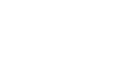
The approach used here generalizes to the multivariate case, by increasing nvar and twonvar and the datafiles. Heath et al. (1989) allow for phenotypic interaction, but this is left for a later example (p. 113)
#Ngroups 3
#define nvar 1 ! number of variables
#define twonvar 2 ! two times nvar
! A C E model fitted to the Heath et al (1989) data on alcohol consumption
G1: model parameters
Calc
Begin Matrices;
X Lower nvar nvar Free ! genetic structure
Y Lower nvar nvar Free ! common environmental structure
Z Lower nvar nvar Free ! specific environmental structure
W Lower nvar nvar Fixed ! dominance structure
H Full 1 1
Q Full 1 1
End Matrices;
Matrix H .5
Matrix Q .25
Begin Algebra;
A= X*X' ;
C= Y*Y' ;
E= Z*Z' ;
D= W*W' ;
End Algebra;
End
G2: Monozygotic twin pairs
Data NInput-vars=twonvar NObservations=171
Labels Alc_t1 Alc_t2
CMatrix
1.28 0.766 1.194
Matrices= Group 1
Covariances A+C+D+E | A+C+D _
A+C+D | A+C+D+E /
Options RSiduals
End
G3: Dizygotic twin pairs
Data NInput_vars=twonvar NObservations=101
Labels Alc_t1 Alc_t2
CMatrix
1.077 0.463 0.962
Matrices= Group 1
Covariances A+C+D+E | H@A+C+Q@D _
H@A+C+Q@D | A+C+D+E /
Start .6 All
Options Multiple RSiduals
End
Power Calculation for the Classical Twin Study
Our next example uses the same model as in the preceding section, but in this case we calculate the power of the classical twin study to detect the effects of common environmental variation. The particular case we wish to examine is where the true population variance comprises 20% additive genetic, 30% shared environment, and 50% random environment variance, but we fit a model without shared environment variation to simulated MZ and DZ covariance matrices. This example is discussed in some detail in Neale & Cardon (1992); here we reproduce their results with a simple script.
There are two stages to the power calculation. First, fixed values of the parameters a, c and e are given, and a two-group Mx script simply calculates the expected covariances under the model, and saves them to two files, mzsim.cov and dzsim.cov. The next problem (preferably in the same input file, though this isn't essential) fits a model of additive genetic and random environmental variance only. The complete input file looks like this:
! A C E model for power calculation
#Ngroups 3
! Step 1: Simulate the data
! 30% additive genetic (.5477�=.3)
! 20% common environment (.4472�=.2)
! 50% random environment (.7071�=.5)
G1: model parameters
Calc
Begin Matrices;
X Lower 1 1 Fixed ! genetic structure
Y Lower 1 1 Fixed ! common environmental structure
Z Lower 1 1 Fixed ! specific environmental structure
H Full 1 1
End Matrices;
Matrix X .5477
Matrix Y .4472
Matrix Z .7071
Matrix H .5
Begin Algebra;
A= X*X' ;
C= Y*Y' ;
E= Z*Z' ;
End Algebra;
End
G2: MZ twin pairs
Calc NInput_vars=2
Matrices= Group 1
Covariances A+C+E | A+C _
A+C | A+C+E /
Options MX%E=mzsim.cov
End
G3: DZ twin pairs
Calc NInput_vars=2
Matrices= Group 1
Covariances A+C+E | H@A+C _
H@A+C | A+C+E /
Options MX%E=dzsim.cov
End
!______________________________________________________________
! Step 2: Fit the wrong model to the simulated data
#Ngroups 3
G1: model parameters
Calc
Begin Matrices;
X Lower 1 1 Free ! genetic structure
Y Lower 1 1 Fixed ! common environmental structure
Z Lower 1 1 Free ! specific environmental structure
H Full 1 1
End Matrices;
Matrix H .5
Begin Algebra;
A= X*X' ;
C= Y*Y' ;
E= Z*Z' ;
End Algebra;
End
G2: MZ twin pairs
Data NInput_vars=2 NObservations=1000
CMatrix Full File=mzsim.cov
Matrices= Group 1
Covariances A+C+E | A+C _
A+C | A+C+E /
Option RSiduals
End
G3: DZ twin pairs
Data NInput_vars=2 NObservations=1000
CMatrix Full File=dzsim.cov
Matrices= Group 1
Covariances A+C+E | H@A+C _
H@A+C | A+C+E /
Start .5 All
Options RSiduals Power= .05,1 ! .05 sig level & 1 df
End
The relevant part of the output is at the end, where we see that for the specified sample sizes of 1000 pairs each of MZ and DZ twins, the 2 goodness-of-fit is 11.35, as found by Neale & Cardon (1992):
Chi-squared fit of model = 11.349
Degrees of freedom = 4
Probability = 0.023
Akaike's Information Criterion = 3.349
Power of this test, at the 0.0500 significance level with 1. df is 0.920572 Based on your combined observed sample size of 2000.
The following sample sizes would be required to reject the hypothesis:
Power Total N
.25 290.
.50 677.
.75 1223.
.80 1383.
.90 1852.
.95 2290.
.99 3238.
Because we requested that this statistic be treated as a 2 for 1 degree of freedom for the purposes of calculating power at the .05 level of significance (Power=.05, 1), the output gives the power of the test given the particular sample sizes (and MZ:DZ sample size proportions), followed by the sample sizes that would be required to obtain certain commonly used levels of power. The power is quite high (.92) with 2000 pairs. The required sample sizes to reach certain power levels from .25 to .99 are also shown.
RAM Specification of Model for Twin Data: Graphics Output
Here is a two group example, a phenotypic interaction PACE model (see page 113 for more details), specified using the three matrix approach of McArdle & Boker (1990). Details of this method, and the syntax of the Draw command can be found on page 101.
The title for the diagram is taken from the title of the group in the Mx input file, and the labels for the variable are taken from labels of the columns of the S matrix. The draw commands in this file produce two files, mx.ram and dz.ram. I don't like the way RAMpath draws interaction between the phenotypes, but there is a certain irrefutable logic in having causal arrows always going out the bottom of a variable and in the top. You can easily edit the RAMpath file to get rid of the @ signs if you like. Note that specifying models à la RAMpath is didactically very clear but computationally inefficient, since the inverse of the maximally dimensioned A matrix is required.
! Phenotypic interaction PACE model, Heath 1989
! Demonstration of RAM specification and output
Group 1: MZ twins
Data NGroups=2 NInput_vars=2 NObservations=171
CMatrix Symm File=alcmz.cov
Matrices
S Symm 8 8
I Iden 8 8
A Full 8 8
F ZIden 2 8
End Matrices;
Matrix S
1
0 1
0 0 1
1 0 0 1
0 1 0 0 1
0 0 0 0 0 1
0 0 0 0 0 0 0
0 0 0 0 0 0 0 0
Label row a a1 c1 e1 a2 c2 e2 p1 p2
Label col a a1 c1 e1 a2 c2 e2 p1 p2
Label row s a1 c1 e1 a2 c2 e2 p1 p2
Label col s a1 c1 e1 a2 c2 e2 p1 p2
Specify A
0 0 0 0 0 0 0 0
0 0 0 0 0 0 0 0
0 0 0 0 0 0 0 0
0 0 0 0 0 0 0 0
0 0 0 0 0 0 0 0
0 0 0 0 0 0 0 0
1 2 3 0 0 0 0 4 ! This is where the parameters are
0 0 0 1 2 3 4 0
Start .6 A 7 1 A 7 3
Covariances F*(I-A)~*S*(I-A)~'*F'/
Options RSiduals Draw=mz.ram
End
Group 2: DZ twins
Data NInput_vars=2 NObservations=101
CMatrix Symm File=alcdz.cov
Matrices
S Symm 8 8
I Iden 8 8
A Full 8 8 = A1
F ZIden 2 8
Matrix S
1
0 1
0 0 1
.5 0 0 1
0 1 0 0 1
0 0 0 0 0 1
0 0 0 0 0 0 0
0 0 0 0 0 0 0 0
Bound -.99 .99 3
Bound 0 5 1 2
Covariances F*(I-A)~*S*(I-A)~'*F'/
Options RSiduals Draw=dz.ram
End
Cholesky Decomposition for Multivariate Twin Data
Any positive definite matrix may be transformed to a product of a lower triangular matrix and its transpose, i.e.
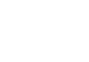
In multivariate genetic analysis, a Cholesky (triangular) decomposition of separate genetic
and environmental covariance matrices is possible. Thus the additive genetic, shared
environment and random environment factors in the simple ACE model (Figure 6.1) have
a multivariate counterpart where the phenotypes ![]() and
and ![]() are replaced by vectors of
observed phenotypes, and the latent variables A, C and E are replaced by vectors of factors.
The path coefficients a c and e are replaced by triangular matrices of factor loadings
according to the Cholesky decomposition. Our aim is to produce a script that is very easy
to modify when the number of variables analyzed changes.
are replaced by vectors of
observed phenotypes, and the latent variables A, C and E are replaced by vectors of factors.
The path coefficients a c and e are replaced by triangular matrices of factor loadings
according to the Cholesky decomposition. Our aim is to produce a script that is very easy
to modify when the number of variables analyzed changes.
Here we use an input file that calculates the genetic, shared and random environmental factors in the first group that generates genetic, shared and random environment covariance matrices It is then a simple matter to form the expected covariance matrices for twin data as partitioned matrices containing linear combinations of these matrices. It is then simplicity itself to fix a parameter to zero, as only one character has to be changed from a 1 to a 0. The example includes data from individuals without cotwins (group 2), as well as MZ (group 3) and DZ (group 4) twin pairs. Estimates from a model such as this depend on the size of the observed variances, and can be difficult to interpret. Estimates of the proportion of variance and covariance due to each source can be obtained using the element division operator (%) (group 5).
! Trivariate Cholesky 'Independent Pathways' model
! Data are Extraversion, Neuroticism and CESD Depression
#Ngroups=5
#Define nvar 3
#Define twonvar 6
#Define nunmatched 449
#Define nMZ 456
#Define nDZ 357
G1: model parameters
Calculation NGroups=5
Begin Matrices;
X Lower nvar nvar Free ! genetic structure
Y Lower nvar nvar Free ! common environmental structure
Z Lower nvar nvar Free ! specific environmental structure
H Full 1 1
End Matrices;
Matrix H .5
Start .6 All
Begin Algebra;
A= X*X' ;
C= Y*Y' ;
E= Z*Z' ;
End Algebra;
End
! Now get to the actual data, and use the results of calculations
G2: Unmatched twins
Data NInput_vars=nvar NObservations=nunmatched
CMatrix Symm File=endun.cov
Matrices= Group 1
Covariances A+C+E /
Option RSiduals
End
G3: MZ twins with cotwins
Data NInput_vars=twonvar NObservations=nMZ
CMatrix File=endmz.cov
Matrices= Group 1
Covariances A+C+E | A+C _
A+C | A+C+E /
Option RSiduals
End
G4: DZ twins with cotwins
Data NInput_vars=twonvar NObservations=nDZ
CMatrix File=enddz.cov
Matrices= Group 1
Covariances A+C+E | H@A+C _
H@A+C | A+C+E /
! By using the Kron operator every element of G is multiplied by .5
Option RSiduals
End
G5: Calculation of standardized solution
Calculation
Matrices= Group 1
I Iden nvar nvar
Begin Algebra;
P= A+C+E;
G= \sqrt(I.P)*A;
K= \sqrt(I.P)*C;
L= \sqrt(I.P)*E;
End Algebra;
Option RSiduals
End
PACE Model: Reciprocal Interaction between Twins
Figure 6.3 shows a path diagram similar to the ACE model for twin data. There is now a path (I) from the phenotype of a twin to that of his or her cotwin. This is reciprocal interaction between dependent variables. It can easily be shown (see appendix D) that a matrix representation of this process is to use the formulation (I B)1, where B is a matrix whose element bjk represents the causal effects of variable k on variable j. In this case, the parameter I has been bounded to lie between -1 and 1, though this is not necessary.
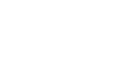
Figure 6.3 PACE model for phenotypic interaction between twins. Path for additive genetic (A), shared environment (C) and specific environment (E) effects on phenotypes (P) of pairs of twins (T1and T2). Path i models direct phenotypic effects of a twin on his or her cotwin. The parameter is fixed at 1 for MZ twins and at .5 for DZ twins.
!Phenotypic interaction model, fit to Heath 1989 data.
#Ngroups 3
G1: model parameters
Calc
Begin Matrices;
X Diag 1 1 Free ! genetic structure
Y Diag 1 1 Free ! common environmental structure
Z Diag 1 1 Free ! specific environmental structure
P Full 2 2 ! interaction parameters
I Iden 2 2
H Full 1 1
End Matrices;
Specify P
0 4
4 0
Matrix H .5
Start .6 All
Bound -.99 .99 4
Bound 0 5 1 2 3
Begin Algebra;
A= X*X' ;
C= Y*Y' ;
E= Z*Z' ;
B=(I-P)~;
End Algebra;
End
G2: female MZ twin pairs
Data NInput_vars=2 NObservations=171
Labels alc_t1 alc_t2
CMatrix Symmetric File=alcmz.cov
Matrices= Group 1
Covariances B &(A+C+E | A+C _
A+C | A+C+E) /
Option RSiduals
End
G3: female DZ twin pairs
Data NInput_vars=2 NObservations=101
Labels alc_t1 alc_t2
CMatrix Symmetric File=alcdz.cov
Matrices= Group 1
Covariances B &(A+C+E | H@A+C _
H@A+C | A+C+E) /
Option RSiduals
Options NDecimals=4
End
Scalar, Non-scalar Sex Limitation and Age Regression
The model and data in this section were taken from Neale & Martin (1989) who fitted a
model of scalar sex-limitation to data from 5 groups of twins who reported subjective
impressions of drunkenness following a challenge dose of alcohol. The model here involves
additive genetic, shared and random environment components (A, C and E; see example on
page 105, and Figure 6.1, but allows these to differ in their effects on the phenotypes of
males and females. In addition, the regression of the phenotypes on Age is modeled, so that
there are parameters for the variance of age (![]() ) and for the regressions (s). A path diagram
of the model is shown in Figure 6.4.
) and for the regressions (s). A path diagram
of the model is shown in Figure 6.4.
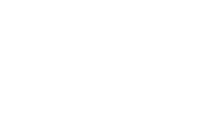
Figure 6.4 Model for sex limitation and age regression. Sex-limited additive genetic (A), shared environment (C) and specific environment (E) effects on phenotypes (P) of pairs of twins (T1 and T2). The parameter is fixed at 1 for MZ twins and at .5 for DZ twins. Either or may be estimated with data from twins, but not both.
Note the use of boundary constraints to prevent the estimation of parameters of opposite sign in the two sexes.
! Age correction
! Sex limitation model
#Ngroups 7
G1: female model parameters
Calculation
Begin Matrices;
X Lower 1 1 Free ! genetic structure
Y Lower 1 1 Free ! common environmental structure
Z Lower 1 1 Free ! specific environmental structure
S Lower 1 1 Free ! effect of age on phenotype
V Lower 1 1 Free ! variance of age
H Full 1 1
End Matrices;
Matrix H .5
Begin Algebra;
A= X*X' ;
C= Y*Y' ;
E= Z*Z' ;
G= S*S' ;
End Algebra;
End
G2: male model parameters
Calculation
Begin Matrices;
X Lower 1 1 Free ! genetic structure
Y Lower 1 1 Free ! common environmental structure
Z Lower 1 1 Free ! specific environmental structure
S Lower 1 1 Free ! effect of age on phenotype
V Lower 1 1 Free ! variance of age
H Full 1 1 =H1
Begin Algebra;
A= X*X' ;
C= Y*Y' ;
E= Z*Z' ;
G= S*S' ;
End Algebra;
End
G3: Female MZ twin pairs
Data NInput_vars=3 NObservations=43
CMatrix Symmetric File=drunkmzf.cov
Labels age drunkt1 drunkt2
Matrices= Group 1
Covariances V*V | S*V | S*V _
S*V | A+C+E+G | A+C+G _
S*V | A+C+G | A+C+E+G /
Option RSiduals
End
G4: Female DZ twin pairs
Data NInput_vars=3 NObservations=44
CMatrix Symmetric File=drunkdzf.cov
Labels age drunkt1 drunkt2
Matrices= Group 1
Covariances V*V | S*V | S*V _
S*V | A+C+E+G | H@A+C+G _
S*V | H@A+C+G | A+C+E+G /
Option RSiduals
End
G5: Male MZ twin pairs
Data NInput_vars=3 NObservations=42
CMatrix Symmetric File=drunkmzm.cov
Labels age drunkt1 drunkt2
Matrices= Group 2
Covariances V*V | S*V | S*V _
S*V | A+C+E+G | A+C+G _
S*V | A+C+G | A+C+E+G /
Option RSiduals
End
G6: Male DZ twin pairs
Data NInput_vars=3 NObservations=38
CMatrix Symmetric File=drunkdzm.cov
Labels age drunkt1 drunkt2
Matrices= Group 2
Covariances V*V | S*V | S*V _
S*V | A+C+E+G | H@A+C+G _
S*V | H@A+C+G | A+C+E+G /
Option RSiduals
End
G7: Female-Male DZ twin pairs
Data NInput_vars=3 NObservations=39
CMatrix Symmetric File=drunkdzo.cov
Labels age drunkt1 drunkt2
Matrices= Group 1
Y Computed 1 1 = G1
J Computed 1 1 = A2
K Computed 1 1 = C2
L Computed 1 1 = E2
X Computed 1 1 = G2
T Lower 1 1 = S2
W Lower 1 1 = V2
Covariances
V*W | S*V | T*W _
S*V | A+C+E+Y | H@(\sqrt(A*J))+Q@(\sqrt(C*K))+(\sqrt(Y*X)) _
T*W |H@(\sqrt(A*J))+Q@(\sqrt(C*K))+(\sqrt(Y*X)) | J+K+L+X /
Start .5 All
Start 10 V 1 1 1 V 2 1 1
Bound 0 5 1 2 3 6 7 8
Option RSiduals
End
Multivariate Assortative Mating: Modeling D
In this section we return to the transformation of the data described on page 102. The question is now, how do we fit a model with parameters in the D matrix, so that we can explore the significance of marital assortment both within and between variables. For example, is there selection of wealthy men by attractive women, or is it just that attractiveness and wealth are correlated, and partners choose each other on the grounds of wealth alone? Neale & McArdle (1990) published a transformation of the matrix equation on page 102 which allowed the fitting of LISREL and COSAN models to marital data. The LISREL implementation of the model is not straightforward, involving phantom latent variables (Rindskopf, 1984). However, the model is very easy to implement in Mx, as is shown below. We have already shown how estimates of parameters in the D matrix may be obtained directly; here we show how to test specific hypotheses about direct and indirect homogamy. Phillips et al. (1988) reports data on general intelligence, educational level, extraversion, anxiety, tough-mindedness and independence in both husbands and wives. The first diagonal element of D therefore represents direct homogamy for intelligence; by fixing this parameter to zero we test the statistical significance of the process.
#Ngroups 1
Assortative mating: Phillips data, Test that D 1 1 is zero
Data NInput_vars=12 NObservations=334
CMatrix File=asmat.cov
Begin Matrices;
H Symm 6 6 Free
W Symm 6 6 Free
D Full 6 6 Free
End Matrices;
Start 1. H 1 1 H 2 2 H 3 3 H 4 4 H 5 5 H 6 6
Start 1. W 1 1 W 2 2 W 3 3 W 4 4 W 5 5 W 6 6
Fix D 1 1
Covariance
H | H*D'*W_
W*D*H | W /
Option RSiduals
End
6.3 Fitting Models with Non-linear Constraints
Any symmetric matrix C may be decomposed to a product ABA where B is a real diagonal matrix and A is a real orthogonal matrix, i.e. AA=I. The elements of B are eigenvalues of C and the columns of A are the eigenvectors of C. In general, if we fitted a model ABA where A was full and B was diagonal, it would be underidentified, since there would be more parameters in the model than in the observed covariance matrix C. However, we can supply the identifying constraints that A is orthogonal. In the Mx input file, these constraints are imposed in group 2, by setting AAI=0. This is not an efficient method of obtaining eigenvalues and eigenvectors of a matrix, but it does highlight non-linearly constrained optimization. For eigenvalue and eigenvector functions, see Table 4.5.
#Ngroups 2
Principal components ABA' with constraints to keep A orthogonal
Data NInput_vars=3 NObservations=100
CMatrix Symm
1.
.6 .9
.4 .2 .7
Matrices
A Full 3 3
B Diag 3 3
Covariances A*B*A'/
Specification A 1 2 3 4 5 6 7 8 9
Specification B 10 11 12
Start 1.0 A(1,1) A(2,2) A(3,3) B(1,1) to B(3,3)
Option LS
End
Here is the constraint A*A'=I
Constraint NInput_vars=3
Matrices
A Full 3 3 = A1
I Identity 3 3
Constraint A*A'=I /
Option LS
End
Analysis of correlation matrices
As Lawley and Maxwell (1971 ch. 7) pointed out, it is incorrect to analyze correlation matrices by maximum likelihood as if they were covariance matrices,. Incorrect analysis leads to biased estimates of the confidence intervals (even the likelihood-based confidence intervals supplied by Mx). Likewise, the goodness-of-fit statistics can be biased, with corresponding bias in the tests of hypotheses that use the likelihood ratio test. These problems are limited to the analysis of correlation matrices using the maximum-likelihood method and do not apply to asymptotic weighted least squares. The easiest way to avoid this problem and one that we most strongly recommend is to fit models to covariance matrices (or raw data) wherever possible.
If it is necessary to fit a model to an observed correlation matrix (perhaps because the correlation matrix is the only available data, possibly published without variances or standard deviations) then Mx can be used for correct analysis. The maximum-likelihood fit function for covariance matrices assumes that the diagonal elements of the covariance matrix are free to vary. If they are all constrained to equal unity, then a modified fit function is required. A simple way to implement this alternative fit function in Mx is to add a constraint group which forces the diagonal elements of the correlation matrix to equal unity, but which does not contribute to the fit function. To illustrate the effects of correct vs. incorrect analysis, we use the data of Lawley and Maxwell (1971). Nine tests of cognitive ability were administered to seventh and eighth grade students by Holzinger and Swineford (1939). The model has three-factors and is shown in Figure 6.4.

Figure 6.5 Three factor model of 9 cognitive ability tests (Lawley & Maxwell, 1971)
Lawley and Maxwell (1971) Analysis of correlation matrix
#Ngroups 2
#include lawley.dat
Begin Matrices;
A Full 9 3
E Diag 9 9 Free
R Stan 3 3 Free
End Matrices;
Label Row E
visperc cubes lozenges parcomp sencomp wrdmng addition cntdot stcurve
Label Col E
visperc cubes lozenges parcomp sencomp wrdmng addition cntdot stcurve
Label Row A
visperc cubes lozenges parcomp sencomp wrdmng addition cntdot stcurve
Label Col A Visual Verbal Speed
Specify A
13 0 0
14 0 0
15 0 0
0 16 0
0 17 0
0 18 0
0 0 19
0 0 20
22 0 21
Start .5 all
Intervals A 4 2 A 5 2 A 6 2
Covariance A&R + E.E;
Options RSidual Multiple
End Group
Constraint Group to make unit diagonal of predicted cov matrix in group 1
Constraint
Matrices = Group 1
B Unit 1 9 ! Matrix of 1's
End Matrices;
! use the \d2v function to extract the diagonal to a vector
Constraint B = \d2v (A&R + E.E') ;
Option df=-9 ! Eliminate degrees of freedom credit for constraints
Option CI=90
End Group
The output with the constraints gives confidence intervals on the loadings from the verbal factor to the verbal tests:
Matrix Element Int. Estimate Lower Upper Lfail Ufail
A 1 4 2 95.0 0.9081 0.8284 0.9727 0 0 0 0
A 1 5 2 95.0 0.8674 0.7774 0.9310 0 0 0 0
A 1 6 2 95.0 0.8241 0.7240 0.8913 0 0 0 0
To compare these results with the incorrect results that do not include the non-linear constraint group, the second group was deleted, and NGroups was reduced to 1. This incorrect analysis gives much larger confidence intervals on the parameters:
A 1 4 2 95.0 0.9081 0.7334 1.1178 0 0 0 0
A 1 5 2 95.0 0.8674 0.6877 1.0816 0 0 0 0
A 1 6 2 95.0 0.8241 0.6402 1.0425 0 0 0 0
Given that these confidence intervals represent approximately 1.96 times the standard errors reported by Lawley and Maxwell, both sets of results closely agree with theirs.
Fitting a PACE Model to Contingency Table Data on MZ and DZ Twins
In order to fit a model with additive genetic, common and specific environment components to categorical data collected from twins, we are faced with two possibilities. One, we could use PRELIS or similar software to estimate tetrachoric or polychoric correlation matrices and associate asymptotic weight matrices, or two, we could fit directly to the contingency tables. Only the latter approach is suitable for models of phenotypic interaction between the twins. Phenotypic interaction leads to different variances between MZ and DZ groups, or in the case of categorical data, to proportionate group differences in the thresholds. This example uses a simple PACE model (see the example shown on page 113) fitted to 2�2 contingency tables obtained from MZ and DZ twin pairs. There is no information on the total variance in these data; but there is information on the relative magnitude of the variance in MZ and DZ groups (via the thresholds). Therefore, it is necessary to constrain the total variance prior to interaction to unity. This is done in the fourth group. Thresholds are constrained equal across groups.
#Ngroups 4
Categorical data analysis. PACE model
Calculation
Begin Matrices;
X Lower 1 1 Free ! genetic structure
Y Lower 1 1 Free ! common environmental structure
Z Lower 1 1 Free ! specific environmental structure
P Full 2 2 ! interaction parameters
I Iden 2 2
T Full 2 1
H Full 1 1
End Matrices;
Specification P 0 4 4 0
Boundary -.99 .99 4
Specification T 5 6
Matrix H .5
Start .6 All
Begin Algebra;
A= X*X' ;
C= Y*Y' ;
E= Z*Z' ;
B=(I-P)';
End Algebra;
End
G2: Monozygotic twin pairs
Data NInput-vars=2
CTable 2 2
File=usmz.ctg
Matrices= Group 1
Thresholds T /
Covariances A+C+E | A+C _ A+C | A+C+E /
End
G3: Dizygotic twin pairs
Data NInput_vars=2
CTable 2 2
File=usdz.ctg
Matrices= Group 1
Thresholds T /
Covariances A+C+E | H@A+C _ H@A+C+| A+C+E /
Options Iterations=300
End
Constraint group to ensure a*a + c*c + e*e = 1
Data Constraint NInput=1
Matrices= Group 1
I Identity 1 1
Begin Algebra;
S= (A|C|E);
End Algebra;
Constraint I = S*S' /
End
Twins and their Parents: Cultural and Genetic Transmission
The model described has been developed extensively in the univariate and multivariate case (Eaves et al., 1978; Fulker, 1982; Neale & Fulker, 1984; Vogler, 1985; Fulker, 1988; Phillips et al., 1988; Cardon, Fulker & Jöreskog, 1991, Neale et al., 1994). In order to preserve consistency with the ACE model presented for twin data alone, the same separation of environmental effects is made here, following the last of the referenced papers instead of the earlier treatments. A path diagram of the model is shown in Figure 6.6.
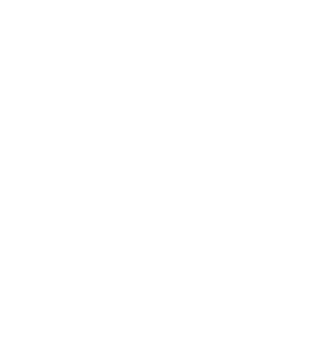
The development of a covariance structure model for this design is not simple. We describe two approaches: (i) direct use of RAM theory in which all variables in the model are represented in two matrices, and the Pearson-Aitken selection formula (see page 104) is used to handle assortative mating, and (ii) an computationally efficient approach that progresses in a stepwise fashion from the top to the bottom of the diagram. Approach (ii) is recommended for general use except where fast hardware gives approach (i) comfortably quick turnaround.
As discussed on page 101, structural equation models may be specified very simply in terms of three matrices. The first matrix, S, is symmetric and specifies all the two-headed arrows between all the variables (both latent and observed) in the diagram. The second matrix, A, is asymmetric and specifies all the single-headed arrows between all the variables in the model. Causal paths from variable i to variable j are specified in element Aji. The third matrix, F, is used to filter the observed variables from the latent variables for the purpose of model fitting. This example is a relatively inefficient approach to fitting this model, but it illustrates the flexibility of Mx to implement theory-driven models explicitly.
! Rose social fears data
! Full 9-Phenotype model for all pedigree types
! P->C transmission & P--P assortment
#Ngroups 6
G1 - covariance in the absence of assortative mating
Calculation
Matrices
A Full 17 17
I Iden 17 17
S Symm 17 17
End Matrices;
Specification A
0 0 0 0 0 1 2 3 0 0 0 0 0 0 0 0 0
0 0 0 0 0 0 0 0 1 2 3 0 0 0 0 0 0
0 0 0 0 0 0 0 0 0 0 0 1 2 3 0 0 0
0 0 0 0 0 0 0 0 0 0 0 1 2 0 3 0 0
0 0 0 0 0 0 0 0 0 0 0 0 2 0 0 1 3
0 0 0 0 0 0 0 0 0 0 0 0 0 0 0 0 0
0 0 0 0 0 0 0 0 0 0 0 0 0 0 0 0 0
0 0 0 0 0 0 0 0 0 0 0 0 0 0 0 0 0
0 0 0 0 0 0 0 0 0 0 0 0 0 0 0 0 0
0 0 0 0 0 0 0 0 0 0 0 0 0 0 0 0 0
0 0 0 0 0 0 0 0 0 0 0 0 0 0 0 0 0
0 0 0 0 0 0 0 0 0 0 0 0 0 0 0 0 0
4 4 0 0 0 0 0 0 0 0 0 0 0 0 0 0 0
0 0 0 0 0 0 0 0 0 0 0 0 0 0 0 0 0
0 0 0 0 0 0 0 0 0 0 0 0 0 0 0 0 0
0 0 0 0 0 0 0 0 0 0 0 0 0 0 0 0 0
0 0 0 0 0 0 0 0 0 0 0 0 0 0 0 0 0
Labels Row A
!1 2 3 4 5 6 7 8 9 10 11 12 13 14 15 16 17
PH PW PMZ1 PMZ2 PDZ AH CH EH AW CW EW AMZ CE EMZ1 EMZ2 ADZ EDZ
Labels Col A PH PW PMZ1 PMZ2 PDZ AH CH EH AW CW EW AMZ CE EMZ1 EMZ2 ADZ EDZ
Value 0.5 A 12 6 A 12 9 A 16 6 A 16 9
Specify S
0
0 0
0 0 0
0 0 0 0
0 0 0 0 0
0 0 0 0 0 0
0 0 0 0 0 8 0
0 0 0 0 0 0 0 0
0 0 0 0 0 0 0 0 0
0 0 0 0 0 0 0 0 8 0
0 0 0 0 0 0 0 0 0 0 0
0 0 0 0 0 0 0 0 0 0 0 5
0 0 0 0 0 0 0 0 0 0 0 0 6
0 0 0 0 0 0 0 0 0 0 0 0 0 0
0 0 0 0 0 0 0 0 0 0 0 0 0 0 0
0 0 0 0 0 0 0 0 0 0 0 0 0 0 0 5
0 0 0 0 0 0 0 0 0 0 0 0 0 0 0 0 0
Labels Col S PH PW PMZ1 PMZ2 PDZ AH CH EH AW CW EW AMZ CE EMZ1 EMZ2 ADZ EDZ
Labels Row S PH PW PMZ1 PMZ2 PDZ AH CH EH AW CW EW AMZ CE EMZ1 EMZ2 ADZ EDZ
Start 1.0 S 6 6 S 7 7 S 8 8 S 9 9 S 10 10 S 11 11 S 14 14 S 15 15 S 17 17
Begin Algebra;
R = (I-A)~ &S ;
End Algebra;
End
Group 2 - Calculations
Calculation
Begin Matrices;
X IZero 2 17
R Comp 17 17 =R1
Y ZIden 17 15
Z ZIden 15 17
I Iden 2 2
M Symm 2 2
End Matrices;
Specify M 0 7 0
Start .1 M 2 1
Begin Algebra;
A= X*R*X' ; ! covariance matrix of parents
B= X*R*Y ; ! covariance of parent phenotypes with other variables
C= Z*R*Z' ; ! covar. of variables that are not parents' phenotypes
D= (A+M)| (A+M)*A~*B _
((A+M)*A~*B)'|C-B'&(A~*(I-(A+M)*A~)); ! handle the effects of assortative mating
End Algebra;
Options RSiduals
End
Group 3 - Constraints on kids' G-E variance and covariance
Constraint
Begin Matrices;
E Computed 17 17 = D2
C Stan 2 2
F Full 2 17
Constraint \vec(F&E)=\vec(C) /
Specify C 8
Matrix F
0 0 0 0 0 0 0 0 0 0 0 1 0 0 0 0 0
0 0 0 0 0 0 0 0 0 0 0 0 1 0 0 0 0
Labels Row F PH PW PMZ1 PMZ2 PDZ AH CH EH AW CW EW AMZ CE EMZ1 EMZ2 ADZ EDZ
Options RSiduals
End
Group 4 - MZ twins & their parents
Data NInput_vars=4 NObservations=144
CMatrix File=usfearmz.cov
Matrices
C Computed 17 17 = D2
F IZero 4 17
Covariances F*C*F'/
Options RSiduals
End
Group 5 - DZ twins & their parents
Data NInput_vars=4 NObservations=106
CMatrix File=usfeardz.cov
Matrices
C Computed 17 17 = D2
F Full 4 17
Covariances F*C*F'/
Matrix F
1 0 0 0 0 0 0 0 0 0 0 0 0 0 0 0 0
0 1 0 0 0 0 0 0 0 0 0 0 0 0 0 0 0
0 0 1 0 0 0 0 0 0 0 0 0 0 0 0 0 0
0 0 0 0 1 0 0 0 0 0 0 0 0 0 0 0 0
Options RSiduals IT=500
End
Group 5 - Summarize parameter estimates
Calculation
Matrices
P Full 1 8
Compute P/
Labels Col P A C E Q ResGs ResCt Mu S
Specification P 1 2 3 4 5 6 7 8
Start .7 P 1 1 P 1 3
Start .5 P 1 5
Start 1 P 1 6
Start .1 P 1 4 P 1 8
End
Computationally Efficient Approach
It is possible to get much faster turnaround with computationally efficient approaches to structural modeling of twins and their parents. In our second script the model for mixed genetic and cultural transmission was specified in terms of the covariances as derived from the rules of path analysis. This is the 'correlational model' described in Neale et al. (1994) but simplified with the algebra syntax. In group 1 all the model parameters are declared in separate matrices. In addition to the A, C and E matrices for additive genetic (A), shared environmental (C) and unique environmental (E) factors, parameters for the residual additive genetic variance (RA), the residual common environmental variance (RC) and the genotype-environment covariance (s) are specified in matrices G, R and S. The genetic transmission paths are fixed to .5 (matrix H). Separate cultural transmission paths are estimated for the maternal (m) and the paternal (p) effects in matrices M and F. The matrix B controls the common environmental residual variance and reflects thus the shared environmental effects of non-parental origin. Assortative mating is modeled as a copath (Eerdewegh, 1982) in matrix D. Matrix P represents the within person covariance. Finally the model allows for non-additive paths (N), but they cannot be estimated simultaneously with the cultural transmission paths in the twin-parent design. The matrices declaration section is ended with the End Matrices; statement, and followed by starting values and boundary constraints for the parameters. Expressions for the expected correlations between the relevant family members (spouses, father-child, mother-child, MZ twin and DZ twin) are given in the multistatement algebra section, indicated by the Begin Algebra; End Algebra; commands.
The model is not identified without nonlinear constraints on certain parameters. These are specified in groups 2 to 5. The within person phenotypic variance is equated to the sum of all genetic and environmental components in group 2. Group 3 equates the genetic variance in children to that of the parents. Similar constraints on the genotype-environment covariance and the environmental variance are calculated respectively in groups 4 and 5.
The observed data are supplied and the fit function is calculated in group 6 for MZ twins and their parents and group 7 for DZ twins and their parents. The expected covariance of these groups is a simple combination of the expected covariances for the respective relationships, as calculated in group 1, using horizontal and vertical adhesion. The only difference between the two groups is the expectation for the covariance between twin 1 and twin 2.
Modifications to the Mx code are relatively simple to make. Additionally, facilities for dropping parameters to fit reduced models or for adding different data summaries make this example a convenient starting point for comprehensive analyses of data from all types of nuclear family and twin and parent data.
! Rose Fear data: Social phobia
! Twins and parents: Genetic and cultural transmission model.
! P--P assortment
#Ngroups 7
G1: Model parameters
Calculation
Begin Matrices;
D Full nvar nvar free ! assortative mating paths
P Symm nvar nvar free ! within person covariance (Rp)
A Low nvar nvar free ! additive genetic paths
C Low nvar nvar free ! common environment paths
F Full nvar nvar free ! paternal cultural transmission
M Full nvar nvar free ! maternal cultural transmission
G Symm nvar nvar free ! additive genetic covariance (Ra)
S Full nvar nvar free ! A-C covariance
R Symm nvar nvar free ! common environment covariance (Rc)
E Low nvar nvar free ! specific environment paths
N Low nvar nvar ! non-additive paths
H Full 1 1 ! scalar, .5
I Iden 1 1 ! identity matrix
B Iden 1 1 ! common env residual variance
End Matrices;
Matrix H 0.5
Start 1.0 P 1 1
Start 1.0 G 1 1
Start .5 A 1 1
Start .5 C 1 1
Start 1.0 R 1 1
Start .707 E 1 1
Bound 0 1 D 1 1 1
Begin Algebra;
W= P*D*P' ; ! Mother-Father Cov
T= G*A' + S*C' ; ! Genotype-Phenotype Cov
O= (P*F'+ W'*M')*C'+ (I+ P*D')*T'*(H@A') ; ! Father-Child Cov
Q= (P*M'+ W*F')*C'+ (I+ P*D)*T'*(H@A') ; ! Mother-Child Cov
J= A*S*C'+ C*S'*A' ;
U= A&G+ C&R+ J + N*N' ; ! MZ Twin
V= H@A*(G+ H@(T&(D'+D)))*A'+ C&R+ J+ H@H@N*N' ; ! DZ Twin
End Algebra;
Option Rsiduals
End
G2: Phenotypic Variance Constraint
Data Constraint NInput=1
Matrices= Group 1
Constraint P- (A&G+ C&R+ E*E'+ A*S*C'+ C*S'*A'+ N*N') /
End
G3: Genetic Constraint
Constraint
Matrices= Group 1
Constraint G= (H@(G+ H@(T*(D'+D)*T')+ I)) /
End
G4: A-C Constraint
Constraint
Matrices= Group 1
Constraint S= (H@T*(M'+ F'+ D*P*M'+ D'*P*F')) /
End
G5: Common Environment Constraint
Constraint
Matrices= Group 1
Constraint R= (M*P*M'+ F*P*F'+ M*W*F'+ F*W'*M'+ B) /
End
G6 - MZ Twins and parents
Data NInput=4 NObservations=144
Labels DAD_1 MOM_1 T1_1 T2_1
CMatrix File=usfearmz.cov
Matrices= Group 1
Covariance ( P | W'| O | P )_
( W | P | Q | Q )_
( O'| Q'| P | U )_
( O'| Q'| U'| P ) /
Option RSiduals
End
G7 - DZ twins and parents Rose Fear Factor 1
Data NInput=4 NObservations=106
Labels DAD_1 MOM_1 T1_1 T2_1
CMatrix File=usfeardz.cov
Matrices= Group 1
Covariance ( P | W'| O | P )_
( W | P | Q | Q )_
( O'| Q'| P | V )_
( O'| Q'| V'| P ) /
Option Rsiduals
Option Iterations=800
Option Multiple
End
! Re-fit model with father-child and mother child cultural transmission set equal
Equate F 1 1 1 M 1 1 1
End
6.4 Fitting Models to Raw Data
When models are fitted to raw data, it is normal to provide a model for the means as well as for the covariances. Otherwise, there is little difference in the approaches. Mx computes minus twice the log-likelihood of the data, with an arbitrary constant that is a function of the data. Thus there is no overall measure of fit, but there are relative measures of fit, since differences in fit function between submodels are distributed as 2.
Estimating Means and Covariances
This section demonstrates maximum likelihood estimation using complete, balanced raw data. A Cholesky decomposition (see Figure 6.2) is used for the covariance structure, and the means are estimated separately. Alternative models for covariances or means or both could be used if desired.
!
! ML fitting to raw data simulated
! with SAS, whose PROC COR COV gave:
! VARIABLE N MEAN STANDARD
! DEVIATION
! P1 1000 0.00182388 0.98499439
! P2 1000 -0.98608262 1.40083917
! P3 1000 2.05400385 1.79139557
!
! COVARIANCE MATRIX
! P1 P2 P3
! P1 0.970214 0.506058 0.620529
! P2 0.506058 1.96235 0.807754
! P3 0.620529 0.807754 3.2091
!
! Cholesky for covariance structure
ML example, calculation of likelihood for each observation.
Data NInput_vars=3 NObservations=1000 NGroups=1
Rectangular File=mlped.raw
Begin Matrices;
M Full 1 3 Free
S Lower 3 3 Free
End Matrices;
Matrix_Start_values S
1
.6 .8
.6 .0 .8
Means M /
Covariances S*S' /
End
The relevant part of the output from this job shows good agreement with the SAS results, calculating means and covariances in the usual fashion, as would be expected for a sample size of 1000. The estimates of the variances are slight underestimates since the ML estimate of a variance is biased, having denominator n instead of n-1. Multiplying the ML estimates by 1000/999 we recover the calculated covariances precisely.
ML EXAMPLE, CALCULATION OF LIKELIHOOD...
Matrix M
This is a FULL matrix of order 1 by 3
0.0018 -0.9861 2.0536
Matrix S
This is a constrained a FULL matrix of order 3 by 3
0.9692 0.5056 0.6199
0.5056 1.9604 0.8069
0.6199 0.8069 3.2059
When there are many different possible configurations of data, it is most convenient to use a variable length data file (see page 43). This information can be read by Mx and the likelihood of the data may be calculated for any structural model for the covariances and the means. In this example, a Cholesky decomposition (see Figure 6.2) of the expected covariance matrix is specified in Group 1.
! ML fitting to variable length data
! Cholesky decomposition for the expected covariance matrix
! Also matrix expression for means
! - in this case just a simple vector with free parameters
Variable pedigree size ML example
Data NInput_vars=3 NObservations=1000 NGroups=1
VLength File=unbal.raw
Begin Matrices;
M Full 1 3 Free
S Lower 3 3 Free
End Matrices;
Start .7 S 1 1 - S 3 3
Means M /
Covariances S*S' /
End
Typical lines of the data file unbal.raw look like this:
2
1 2 0.5550 -1.1114
3
1 2 3 1.6442 -0.1319 3.609508
3
1 2 3 -0.2145 -1.2193 5.011667
3
1 2 3 2.2274 -1.9423 0.714351
There can be problems when beginning to fit models to VL data. One commonly encountered difficulty is that at the starting values, the likelihood is effectively zero for one or more pedigrees. Since Mx is going to try to take the logarithm of the likelihood, some corrective action is required. During iteration a penalty function is used, but this doesn't help the case where there are poor starting values. To help guide the user to the problem with the starting values, Mx prints out 3 columns of information: the observed and expected means, and then the standardized difference between them. Now if these differences are large (say more than 3 for any variable), it would be a good idea to change starting values of either the means (to make the expected ones closer to the observed) or the variances (to make the standardized difference less). If the starting values of the means are very bad, then it would make sense to change them; however, if they are not, the error may occur with another vector in the dataset, in which case modifying the starting values to increase the expected variances should help. If not, examine the expected covariance matrix; sometimes large expected covariances can make particular pairings of scores rather unlikely. It is usually better to supply starting values that specify a diagonal variance-covariance matrix, since the overall likelihood is simply the product of the likelihoods of the individual variables. If each of these likelihoods is reasonable, e.g. a standardized difference of less than 2, then the overall likelihood will not produce problems unless the number of variables in the vector is large.
For example: suppose that the variances of and covariance between two variables vary as a function of age. A traditional approach to this problem might involve splitting the sample into two groups, young and old, and fitting a two-group model. Comparison of the fit statistic obtained when the covariance is constrained to be equal in the two groups to that obtained when each group has its own covariance structure provides a test of heterogeneity. But what if we want to use all the information on age, which is a continuous variable, instead of an arbitrary cutoff for young vs. old?
We can use the observed age variable to define the covariance structure for that particular observation. That is, we want to fit a model of the form
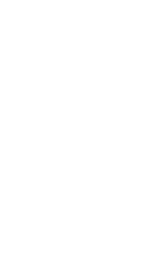
Figure 6.7 Definition variable example.
Title - verbal and performance IQ covariance as a function of age
Data NInput=3 NGroups=1 ! Single group example with 3 variables
Labels Verbal Quant Age
VL file=IQ.VL
Definition_variables Age / ! This variable is referenced as -1 in
! specification statements
Matrices
L Lower 2 2 Free ! Triangular matrix of paths from factor Fi to variable Oj
X Lower 2 2 Free ! Triangular matrix of paths from factor Ai to variable Oj
R Diag 2 2 ! Matrix for variances of Ai latent variables
M Full 1 2 Free ! Matrix for estimating means
Means M / ! Formula to compute mean vector
Covariance L*L' + X*R*X' / ! Formula to compute covariances
Specify R -1 -1 ! Place definition variable on the diagonal elements of R
Matrix M 100 100 ! Starting values for means
Matrix L 15 0 15 ! Starting values for constant covariance component
Matrix X 3 0 3 ! Starting values for age-dependent covariance component
Option RSiduals ! Request some output
End
Internally, Mx will recalculate the predicted covariance matrix for every observation(10). The usual raw data log-likelihood function is computed for every vector of observations, but using the appropriate covariance matrix for this group. If we were to assign one and zero to the age variable in accordance to our cutoff approach, we would get the same results as the two-group heterogeneity method.
Apart from this handling of continuous heterogeneity, we should be aware that considerably more complex models may be attacked. All the tools of Mx matrix functions and operators may be used to define linear and non-linear functions of the definition variables and model parameters.
Using NModel to assess heterogeneity
Mx has special features for assessing possible mixtures of distributions. Almost all structural equation models make the implicit assumption that one model describes the whole population. In reality, the population may consist of several subpopulations. This type of analysis requires the raw data to be analyzed, and thus assumes a multivariate normal distribution of each of the component subpopulations. The likelihood function is modified for this type of mixture. Let L1 be the likelihood under model 1 and L2 be the likelihood under model 2. In both cases, this likelihood is computed with the multivariate normal probability density function, as described on page 63. The overall likelihood is computed as a weighted sum of the likelihoods for each model, and the log-likelihood is the logarithm of this overall likelihood. Mx lets you enter any matrix formula for the weights; here we illustrate the method with a simple proportion.
Suppose that the population consists of a mixture of two groups, one with population covariance matrix
Using SAS, a data set of 500 pairs of scores for each of the two groups was simulated. In addition, two further scores were added to the dataset: (i) a measure of group membership, being N(0,1) for the first group, and N(1,1) on the second a normally distributed indicator with a 1 standard deviation difference between the groups; and (ii) a key variable scored 0 for the first group and 1 for the second. The observed covariance matrices for the two groups and the recovered estimates for a variety of models are shown in Table 6.1. First, the results of fitting a model with no heterogeneity. The covariance is estimated at .47 which is approximately half way between .2 and .8 simulated for the two populations. Second are the results of attempting to detect this heterogeneity with a simple model that tries to estimate the proportions in the two samples. There is evidence of heterogeneity here, because the fit function has improved compared to model 1. However, the parameter estimates recovered are not good estimates of the population statistics, particularly for the low correlation group, whose proportion is estimated at only .27 of the population. Better estimates are recovered when the true population proportion is used (Fixed Heterogeneity model). Therefore, without external indicators, it seems dangerous to draw conclusions about the proportions in the population, unless sample sizes are much larger than they are here. The Fixed Indicator model uses the information from the indicator variable to partially discriminate between the populations. A better fit is found, and good recovery of the population parameters is obtained. To make this model realistic, the relationship between the indicator and group membership should be estimated. Again, the parameter estimates are less realistic, particularly for the less correlated subpopulation, when the proportions are estimated rather than given.
In summary, it may be possible to detect the presence of heterogeneity in a raw dataset with a moderately large sample size. However, unless one has a good indicator variable - and knows its relationship to the variables being analyzed - it is difficult to quantify the way in which the 'latent groups' differ. One example where a good indicator variable is available is genetic linkage (Eaves et al., 1996). Modeling heterogeneity with and without indicators is in need of further study, both the complexity of the models used, and the sample proportions.
Table 6.1 Summary of parameter estimates for a variety of models of heterogeneity
| Model | V1 | C | V2 | p | -2ln L | df |
| One model | 1.0093 | 0.4699 | 0.8394 | 5344.12 | 1995 | |
| Estimated
Heterogeneity |
0.5949
1.1779 |
-0.1968
0.7259 |
1.0359
0.8840 |
0.2727 | 5289.39 | 1991 |
| Fixed
Heterogeneity |
0.8409
1.1957 |
0.1353
0.8113 |
1.0065
0.8449 |
.5000 | 5293.28 | 1992 |
| Fixed
Indicator |
0.9460
1.0920 |
0.1721
0.7764 |
0.9830
0.8679 |
5267.59 | 1995 | |
| Estimated
Indicator |
0.6794
1.1672 |
-0.1476
0.7456 |
1.0017
0.8922 |
5263.80 | 1988 | |
| Perfect
Indicator |
0.9997
1.0393 |
0.1356
0.8125 |
0.8473
1.0036 |
5101.71 | 1992 |
Data were simulated with unit variance and .8 correlations for 500 cases, and unit variance and .2 correlation for 500 cases.
#Ngroups 1
No heterogeneity
Data NInput=4 Nobservations=0
Rectangular File=sim1.both
Labels X Y Z Key
Select X Y /
Begin Matrices;
A Lower 2 2 free
M Full 1 2 free
End Matrices;
Start 1 A 1 1 to A 2 2
Means M ;
Covariance A*A' ;
Option Mx%p=indiv1.lik
End Group;
#Ngroups 1
Simple Heterogeneity - two models, no indicator
Data NInput=4 Nobservations=0 Nmodel=2
Rectangular File=sim1.both
Labels X Y Z Key
Select X Y /
Begin Matrices;
A Lower 2 2 free
B Lower 2 2 free
I Unit 1 1
M Full 1 2 free
P Full 1 1 free ! proportion in subpopulation 1
End Matrices;
Start 1 A 1 1 to A 2 2
Start .5 B 1 1 to B 2 2 P 1 1
Bound .001 .999 P 1 1
Begin Algebra;
Q = I - P; ! proportion in subpopulation 2
W = P _
Q ; ! vector of weights
End Algebra;
Means M_M ;
Covariance A*A'_B*B' ;
Weight W ;
Option Mx%p=indiv.lik ! put individual likelihood statistics to file
Option RSiduals Multiple
End Group;
! Fixed proportions heterogeneity
Drop @.5 P 1 1 1
Exit
#Ngroups 1
Estimated indicator
Data NInput=4 Nobservations=0 Nmodel=2
Rectangular File=sim1.both
Labels X Y Z Key
Select X Y Z /
Definition Z /
Begin Matrices;
A Lower 2 2 free ! Cholesky of first subpopulation covariances
B Lower 2 2 free ! Cholesky of second subpopulation covariances
I Unit 1 1
M Full 1 2 free ! Vector of estimated means
C Full 1 1
J Full 1 1 free !Mean of first group on Z variable
K Full 1 1 free !Deviation of Mean of second group
L Full 1 1 free !Variance of first group on Z variable
N Full 1 1 free !Variance of second group on Z variable
End Matrices;
Specify C Z
Start 1 A 1 1 to A 2 2 L 1 1 N 1 1
Start .5 B 1 1 to B 2 2 J 1 1
Start .25 K 1 1
Bound .1 3 L 1 1 N 1 1
Bound 0 3 K 1 1
Bound -3 3 J 1 1
Begin Algebra;
P = \pdfnor(C_J+K_N) % ( \pdfnor(C_J_L) + \pdfnor(C_J+K_N) ) ; ! compute prob
Q = I - P;
W = P _ Q ;
End Algebra;
Means M_M ;
Covariance A*A'_B*B' ;
Weight W ;
Option Mx%p=indiv.lik
Option RS
End Group;
#Ngroups 1
Fixed indicator
Data NInput=4 Nobservations=0 Nmodel=2
Rectangular File=sim1.both
Labels X Y Z Key
Select X Y Z /
Definition Z /
Begin Matrices;
A Lower 2 2 free
B Lower 2 2 free
I Unit 1 1
M Full 1 2 free
C Full 1 1
Z Zero 1 1
End Matrices;
Specify C Z ! put individual Z variable scores into matrix C
Start 1 A 1 1 to A 2 2
Start .5 B 1 1 to B 2 2
Begin Algebra;
P = \pdfnor(C_I_I) % ( \pdfnor(C_Z_I) + \pdfnor(C_I_I) ) ;
! P computes probability separately for every case in the sample
Q = I - P;
W = P _
Q ;
End Algebra;
Means M_M ;
Covariance A*A'_B*B' ;
Weight W ;
Option Mx%p=indiv.lik
Option RS
End Group;
#Ngroups 1
Two groups, perfect indicator (Key)
Data NInput=4 Nobservations=0 Nmodel=2
Rectangular File=sim1.both
Labels X Y Z Key
Select X Y Key /
Definition Key /
Begin Matrices;
A Lower 2 2 free
B Lower 2 2 free
F Full 1 1
I Unit 1 1
M Full 1 2 free
C Full 1 1
Z Zero 1 1
End Matrices;
Specify C Key
Matrix F 5
Start 1 A 1 1 to A 2 2
Start .5 B 1 1 to B 2 2
Begin Algebra;
P = C ; ! compute prob
Q = I - P;
W = P _
Q ;
End Algebra;
Means M_M ;
Covariance A*A'_B*B' ;
Weight W ;
Option Mx%p=indiv.lik
Option RS
End Group;
6.5 User-Defined Fit Functions
This is a simple example to illustrate the use of a user-defined fit function, in this case least-squares. The model statement evaluates to a scalar which is minimized by Mx. Note that this approach is generally less efficient than using built-in formulae available in Mx, but it is much more flexible.
User defined function to fit to a correlation matrix by least squares
Data NInput_vars=3 NGroupies=1
CMatrix Symm
1
.2 1
.3 .4 1
Begin Matrices;
A Symm 3 3 = %O1
B Stan 3 3 Free
End Matrices;
Begin Algebra;
D= \vec(A)-\vec(B);
End Algebra;
Compute \sum(D.D);
Option User
End
On page 85, we described how proband-ascertained ordinal data could be used to estimate population covariances or genetically informative parameters. This same truncate selection might be applied using a screening instrument, so that only individuals above a certain threshold value are sampled. If such an ascertainment scheme was applied in a pairwise fashion, such that only pairs in which at least one of the pair was above threshold, the likelihood of these observations would require correction for the necessarily missing pairs concordant for being below threshold. Mathematically, the likelihood of pair ascertainment can be expressed as a double integral of the bivariate normal distribution:


Simulated twin data. Raw ML estimation
Data NInput=2 NGroups=3 NObservations=1000
Raw_data file=[neale.sas]mzasc.dat
Begin Matrices;
M Full 1 2
R Stan 2 2 Free
End Matrices;
Mean M /
Covariance R /
Matrix M 0 0
Bound -.99 .99 R 1 2
Option RSiduals
End
Dummy group to calculate expected cell proportions
Data NInput=2
CTable 2 2
0 0
0 0 ! It's full of zeros so it contributes zero to the function
Begin Matrices;
T Full 2 1
R Stan 2 2 = R1
End Matrices;
Matrix T
1.282 1.282
Thresholds T /
Covariance R /
Option RSiduals
End
Calculate ascertainment correction
Data NInput=0
Begin Matrices;
I Iden 1 1
J IZero 1 2
P Full 2 2 = %P2
T Full 1 1
End Matrices;
Matrix T 2000 ! twice the sample size of group 1
Compute T*\ln(I-J*P*J') /
Options User-defined RSiduals Multiple
End
Appendix A Using Mx under different operating systems
Currently the Mx statistical engine is available for several Unix systems including Linux, Solaris, Irix, IBM AIX, Digital Unix, HP Ux). Versions for most operating systems can be downloaded via the internet at http://views.vcu.edu/mx. The Mx Graphical Interface (MxGui) is available for MS Windows and MS-DOS and may be obtained from http://www.vipbg.vcu.edu/mxgui. It can use either the included DOS version or Unix version to analyze data.
To run the Mx graphical interface, you need:
To use networked Unix workstations to run the Mx statistical engine (for faster turnaround of cpu intensive jobs) a TCP/IP connection is needed.
Windows 95/98/NT
Download mxgui95.zip and unzip it into a directory such as c:\temp1 (alternatively you can use WinZip http://www.winzip.com to unzip and install in a single step). Run the program setup.exe by double-clicking on it in the Windows Explorer and follow the instructions for the installation. Choose an installation directory that is different from the directory containing the setup.exe program.
Windows 3.xx
Download the file mxgui31.zip and unzip it into a directory such as c:\temp1 (alternatively you can use WinZip http://www.winzip.com to unzip and install in a single step). Run the setup.exe file by double clicking on it in the File Manager and follow the instructions for the installation. Choose an installation directory that is different from the directory containing the setup.exe program; we recommend the default C:\mxgui.
See Chapter 2.
Dos
Mx is written in about 30,000 lines of FORTRAN, and it links to a further 20,000 lines of NPSOL code for optimization, so the resultant .exe file does not run within the 640K limit. Fortunately, the Lahey compiler allows binding of a loader to the code which permits Mx to use memory beyond the 640K limit in 386 and 486 machines. If the program runs out of memory, it will use virtual memory (disk space) instead, but obviously this can drastically decrease performance. The use of Stacker (file compression software) also seems to slow things down, especially for the first run in a multiple fit file. Under DOS, performance can be improved if SMARTMEM is loaded.
Note the difference between your computer running out of memory and Mx running out of workspace. Currently, the PC version is configured with 100,000 double precision words of workspace; larger workspace can be requested on the command line with e.g.
mx -k 500
which would request 500,000 words of workspace.
We recommend that input files have the naming convention cutename.mx where cutename is a name of your choice. To run Mx on a PC, create an input script and type
mx cutename.mx {cutename.mxo}
if you are running DOS. Mx now no longer requires that the output files be specified on the command line. With the syntax
mx cutename.mx
the output will be in a file called cutename.mxo
If you wish to use other extensions or names for input and output files, you could, for example, create a file called badname.abc, and use the syntax:
mx badname.abc awfulname.xyz
which would create an output file called awfulname.mxo. The command
mx badname.abc
would generate an output file called badname.mxo
UnderWindows 3.x, 95 and NT, it is handy to use the Associate option in the File Manager, to associate .mx files with the mx.exe program file. Double-clicking a .mx file will then run Mx and produce a .mxo output file. Feedback of function evaluations is printed on the screen. Alternatively the input file can be launched on the Mx icon. Similarly the .mxo files can be associated with your favorite text editor/viewer, so that output files are easily read with a double click.
We can extend the idea of filename extensions a little further to include: covariance matrices, .COV; correlation matrices, .COR; contingency tables, .CTG; matrices, .MAT; variable length files, .VL; rectangular files, .REC; weight matrices, .ASY; inverted weight matrices, .ASI; vectors of means, .MEA; mx save files, .MXS. Of course, it doesn't make any difference to the program what you call the files, but some widely-used conventions such as these help you and other users to understand the content of the directory when you (or your colleagues) look at it six months later.
Hypertext output may be requested with the -h flag, e.g.
mx -h myfile.mx myfile.htm
would produce html output suitable for looking at with a browser like Netscape.
Mx may be used very simply in UNIX by typing
mx <inputfile >outputfile
and the parameter & may be added to run jobs in batch. For very cpu intensive applications the command
nice mx <inputfile >outputfile
may be used to run the job at lower priority to avoid overtaxing the system.
You can also use a bmx script which allows you to use the following syntax:
bmx inputfile
The outputfile is then automatically created as inputfile.mxo; the bmx script may be downloaded, but it is quite short:
(usr/local/bin/mx <$1.mx >$1.mxo; \
echo "Mx has just finished a job for you ^G"; \
echo "See output in $1.mxo")
and should be entered as a single line, with the literal character ctrl-G (ASCII code 7) to make a beep.
The VMS version is no longer supported; however, version # is still available at the website. Mx for VMS is distributed with a command file (MX.COM) which deals with file extensions and checks to see whether the user has sufficient memory resources. Typically one user at a site, the administrator, will keep the command and executable files with read and execute permission set for all users. Then if users define the symbol mx with a command such as
$ MX :== "@DISK1:[BOSS.MX]MX.COM DUMMY"
where DISK1 is the name of the diskdrive, BOSS is the name of the administrator, and BOSS.MX is the name of the subdirectory in which the mx.com and mx.exe files are stored. The above symbol definition will permit users to run Mx either interactively or as a batch job. The only difference is that the former will produce a mesmerizing display of the Mx logo and the latter will free up your terminal to do something else while it runs. The output file may be read while the program is running, though emptying the print buffer has been reduced to improve performance.
Mx can be run either interactively with the following syntax:
$ MX CUTENAME
or alternatively, you can run the job in batch with
$ BAT/Q=whateveryoulike MX CUTENAME
for short jobs, ignore the /Q= bit. With this syntax, the output will be called CUTENAME.MXO.
There is also a facility , called imx, for editing jobs, running them, and viewing the output.
If, while looking for a number, a (non-comment) input line with only non-numeric characters on it (e.g. matrix P) is found, the program issues a warning:
**WARNING** Non-numeric characters found when trying to read a number
This is to alert the user to what is probably an error of not reading enough numbers, for one of these reasons:
This is not a fatal error, but normally some other problem will arise. Similarly, if too many numbers have been provided for a matrix, (or a mistake was been made when defining the type or dimensions of the matrix) the program will usually try to read a number as a keyword, ask something like "Just what is this keyword supposed to mean?'" and stop.
Sometimes an integer overflow will occur if too many digits have been read in free format for a number. Try to keep the number of digits to 9 or less. If you really need more precision, use the exponential format (D+00) or read data from a file.
This is a list of the error codes reported by Mx. The error messages are supposed to be self-explanatory, but they are usually quite brief. Here the italic text is the error, and ordinary type gives a little further explanation.
Some of these error messages are a little informal. I apologize. I'm terribly terribly sorry and I won't do it again.
What I am really sorry about is if Mx gives you the wrong error message. This is quite rare, but occasionally it is possible to screw up memory, and one of the sensitive areas is the matrix formula. When this has occurred, you may see
"Dump of formula being calculated"
while the program is running. It is important to check the formulae, but if they seem ok, it's time to email technical support. One untrapped source is if you say
Start .5 A 1 2 3 to A 2 2 3
in which case everything between the memory addresses of A of group 1 and A of group 2 gets overwritten with .5. A little care can go a long way; so can a little more foolproof programing which I shall try to provide as soon as I can. Please let me know of any nonsensical error messages that you get; elucidation is prerequisite for elimination.
Appendix C Introduction to Matrices
A matrix is a table of numbers or symbols laid out in rows and columns, e.g.

It is conventional to specify the configuration of the matrix in terms of Rows�Columns and these are its dimensions. Thus the first matrix above is of dimensions 3 by 2 and the second is a 3�3 square matrix.
The most common occurrence of matrices in behavioral sciences is the data matrix where the rows are subjects and the columns are measures. e.g.

Thus we might say that our data matrix is A, which in handwriting we would underline with either a straight or a wavy line. Sometimes a matrix may be written 4A2 to specify its dimensions. When a matrix consists of a single number, it is called a scalar; when it consists of single column (row) of numbers it is called a column (row) vector. Vectors are normally represented as a bold lowercase. Thus the weights of our four subjects are

Matrix algebra defines a set of operations that may be performed on matrices. These operations include addition, subtraction, multiplication, inversion (multiplication by the inverse is similar to division) and transposition.
A matrix is transposed when the rows are written as columns and the columns are written as rows. This operation is denoted by writing A or AT. In our example,
The Mx script would look as follows:
Title: transpose of matrix A
Calculation NGroups=1
Begin Matrices;
A Full 4 2
End Matrices;
Matrix A
50 20
100 40
150 60
200 80
Begin Algebra;
B= A';
End Algebra;
End
Matrix Addition and Subtraction
Matrices may be added and to do so they must be of the same dimension. They are then said to be conformable for addition. Each element in the first matrix is added to the corresponding element in the second matrix to form the same element in the solution, e.g.

You cannot add


Matrices may be multiplied and to do so they must be conformable for multiplication. This means that adjacent columns and rows must be of the same order. For example, the matrix product 3A2�2B2 may be calculated; the result is a 3�2 matrix. In general, if we multiply two matrices iAj�jBk, the result will be of order i�k.
Matrix multiplication involves calculating a sum of cross products among rows of the first matrix and columns of the second matrix in all possible combinations, e.g.

The only exception to the above rule is multiplication by a single number called a scalar. Thus for example,

It is not possible to use this convention directly in Mx; however, it is possible to define a 1�1 matrix with the constant 2.0 as the sole element, and use the kronecker product.
The simplest example of matrix multiplication is to multiply a vector by itself. If we premultiply a column vector by its transpose, the result is a scalar called the inner product. For example, if


![]() ,
which is the square root of the inner product of the vector.
,
which is the square root of the inner product of the vector.
Multiplication Exercises
Try these exercises either by hand, or using Mx, or both, as suits your needs.
Let
Let
Let
C.3 Equations in Matrix Algebra
Matrix algebra provides a very convenient short hand for writing sets of equations. For example, the pair of simultaneous equations


"Real variables (y) = matrix � hypothetical variables."
To show the simplicity of the matrix notation, consider the following equations:


C.4 Calculation of Covariance Matrix from Data Matrix
Suppose we have a data matrix A with rows corresponding to subjects and columns corresponding to variables. We can calculate a mean for each variable and replace the data matrix with a matrix of deviations from the mean. That is, each element aij is replaced by aij�j where �j is the mean of the jth variable. Let us call the new matrix X. The covariance matrix is then simply calculated as:
For example, suppose we have the following data:


Transformations of Data Matrices
Matrix algebra provides a natural notation for transformations. If we premultiply the matrix iBj by another, say kTi, then the rows of T describe linear combinations of the rows of B. The resulting matrix will therefore consist of k rows corresponding to the linear transformations of the rows of B described by the rows of T. A very simple example of this is premultiplication by the identity matrix (written I), which merely has 1's on the leading diagonal and zeroes everywhere else. Thus the transformation described by the first row may be written as 'multiply the first row by 1 and add zero times the other rows.' In the second row, we have 'multiply the second row by 1 and add zero times the other rows,' and so the identity matrix transforms the matrix B into the same matrix. For a less trivial example, let our data matrix be X, then


For a square matrix A we may calculate a scalar called the determinant which we write as |A|. In the case of a 2�2 matrix, this quantity is calculated as

To calculate the determinant of larger matrices, we employ the concept of a cofactor. If we delete row i and column j from an n� n matrix, then the determinant of the remaining matrix is called the minor of element aij. The cofactor, written Aij is simply:
The determinant of a matrix is related to the concept of definiteness of a matrix. In general, for a null column vector x, the quadratic form xAx is always zero. For some matrices, this quadratic is zero only if x is the null vector. If xAx>0 for all non-null vectors x then we say that the matrix is positive definite. Conversely, if xAx<0 for all non-null x, we say that the matrix is negative definite. However, if we can find some non-null x such that xAx=0 then the matrix is said to be singular, and its determinant is zero. As long as no two variables are perfectly correlated, and there are more subjects than measures, a covariance matrix calculated from data on random variables will be positive definite. Mx will complain (and rightly so!) if it is given a covariance matrix that is not positive definite. The determinant of the covariance matrix can be helpful when there are problems with model-fitting that seem to originate with the data. However, it is possible to have a matrix with a positive determinant yet which is negative definite (consider -I with an even number of rows), so the determinant is not an adequate diagnostic. Instead we note that all the eigenvalues of a positive definite matrix are greater than zero. Eigenvalues and eigenvectors may be obtained from software packages and the numerical libraries listed above(11).
Just as there are many uses for the operation of division in ordinary algebra, there are many valuable applications of the inverse of a matrix. We write the inverse of the matrix A as A1, and one of the most important results is that
Procedure for Inversion of a General Matrix
In order to invert a matrix, the following four steps can be used:
For example, the matrix


To verify this, we can multiply AA1 to obtain the identity matrix:


For a larger matrix it is more tedious to compute the inverse. Let us consider the matrix

1. The determinant is


Appendix D Reciprocal Causation
Consider the Path Diagram in Figure D.1.
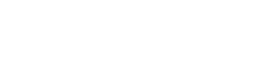
Figure D.1 Feedback loop between two variables, x1 and x2.
This shows a feedback loop between two internal variables, which we call x variables. The total variance of x1 and x2 is the sum of the infinite geometric series:

This formula generalizes to the case of a matrix of such effects between more than a pair of variables (Jöreskog & Sörbom, 1989). In general
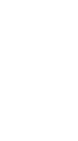
Figure D.2 Structural equation model for x variables
Algebraically, the model for the x variables is:


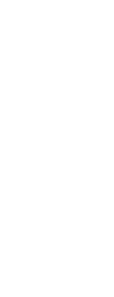
The algebra for the covariance of the observed variables, y, is very similar.

Appendix E Frequently Asked Questions
Here is a list of some of the frequently asked questions about Mx GUI.
Aitken, A.C. (1934). Note on selection from a multivariate normal population. Proceedings of the Edinburgh Mathematical Society B 4:106-110.
Aitken, A.C. (1934-35). On least squares and the linear combination of observations. Proceedings of the Royal Society of Edinburgh 55:42-48.
Akaike, H. (1987). Factor analysis and AIC. Psychometrika 52:317-332.
Bentler, P.M. (1989). EQS Structural Equations Program Manual. Los Angeles: BMDP.
Bentler, P.M. and Bonett, D.G. (1980). Significance tests and goodness of fit in the analysis of covariance structures. Psychological Bulletin 88: 588-606.
Bollen, K.A. (1992). Structural Equations with Latent Variables. New York: Wiley.
Browne, M.W. (1974). Generalized least squares estimators in the analysis of
Covariance structures. South African Statistical Journal 8:1-24.
Browne, M.W. (1982). Covariance structures. In D.M. Hawkins (ed.): Topics in applied multivariate analysis. Cambridge: Cambridge University Press.
Browne, M.W. (1984). Asymptotically distribution-free methods for the analysis of
Covariance structures. British Journal of Mathematical and Statistical Psychology 37:1-21.
Browne, M.W. and Cudeck, R. (1990). Single sample cross-validation indices for
Covariance structures. Multivariate Behavioral Research 24:445-455.
Bryk, A.S. & Raudenbush, S.W. (1992) Hierarchical Linear Models: Applications and data analysis methods. Newbury Park: Sage Press.
Cardon, L.R., Fulker, D.W. & Jöreskog, K. (1991). A LISREL model with constrained parameters for twin and adoptive families. Behavior Genetics 21:327-350.
Carey, G. (1986). A general multivariate approach to linear modeling in human genetics. American Journal Human Genetics 39:775-786.
Eaves, L.J., Last, K., Young, P.A., Martin, N.G. (1978). Model fitting approaches to the analysis of human behaviour. Heredity 41:249-320.
Eaves, L.J., Neale, M.C., Maes, H. (1996). Multivariate multipoint linkage analysis of Quantitative Trait Loci. Behavior Genetics 26: 519-525.
Everitt, B.S. (1984). An introduction to latent variables models. London, New York: Chapman and Hall.
Fraser, C. (1988). COSAN User's Guide Unpublished documentation, Centre for Behavioural Studies in Education, University of New England, Armidale NSW Australia 2351.
Fulker, D.W. (1982). Extensions of the classical twin method. In Human genetics, part A: The unfolding genome (pp. 395-406). New York: Alan R. Liss.
Fulker, D.W. (1988). Genetic and cultural transmission in human behavior. In: B.S. Weir, E.J. Eisen, M. Goodman & G. Namkoong (eds.) Proceedings of the Second International Conference on Quantitative Genetics Massachusetts: Sinauer Associates Inc.
Genz, A. (1992) Statistics applications of subregion adaptive multiple numerical integration. In: T.O. Espelid, A. Genz, (eds.) Numerical Integration (pp. 267-280). Dordrecht, NL:. Kluwer Academic Publishers.
Heath, A.C., Neale, M.C., Hewitt, J.K., Eaves, L.J., & Fulker, D.W. (1989a). Testing structural equation models for twin data using LISREL. Behavior Genetics, 19:9-36.
Heath, A.C., Eaves, L.J., & Martin, N.G. (1989b). The genetic structure of personality III. Multivariate genetic item analysis of the EPQ scales. Personality and Individual Differences 10:877-888.
Hopper, J.L. & Mathews, J.D. (1982). Extensions to multivariate normal models for pedigree analysis. Ann. Hum. Genet. 46:373-383.
Horn, J. & McArdle, J.J. (1992) A practical and theoretical guide to measurement invariance in aging research. Experimental Aging Res 18:117-144.
Johnson, N.I. & Kotz, S. (1970). Distributions in Statistics: Continuous Univariate Distributions 1. Boston: Houghton Mifflin.
Jöreskog, K.G. (1967). Some contributions to maximum likelihood factor analysis. Psychometrika 32:443-482.
Jöreskog, K.G. & Goldberger, A.S. (1972). Factor analysis by weighted least squares. Journal of the American Statistical Association 10:631-639.
Jöreskog, K.G. (1973). A general method for estimating a linear structural equation system. In: A.S. Goldberger & O.D. Duncan (Eds.) Structural equation models in the social sciences. New York: Seminar Press.
Jöreskog, K.G. & Sörbom, D. (1986). PRELIS: A Preprocessor for LISREL. Scientific Software: Mooresville, Indiana.
Jöreskog, K.G. & Sörbom, D. (1989). LISREL 7: A Guide to the Program and Applications 2nd Edition. Chicago, Illinois: SPSS Inc.
Jöreskog, K.G. & Sörbom, D. (1993). New features in PRELIS 2 Chicago: Scientific Software International, Inc.
Kaplan, D. (1990). Evaluating and modifying covariance structure models: A review and recommendation. Multivariate Behavioral Research 25:137-155.
Karlin, S., Cameron, E.C. & Chakraborty, R. (1983). Path analysis in genetic epidemiology: A critique. American Journal of Human Genetics 35:695-732.
Kendall, M., Stuart, A. (1977). The advanced theory of statistics. New York: Macmillan.
Lange, K., Westlake, J., Spence, M. (1976). Extensions to pedigree analysis: III. Variance components by the scoring method. Annals of human genetics 39:485-491.
Little, R.J.A. & Rubin, D.B. (1978) Statistical Analysis with Missing Data. New York: Wiley and Son.
Loehlin, J.C. (1987). Latent variable models. Baltimore: Lawrence Erlbaum Associates.
Marsh, H.W., Balla, J., Hau, K.T. (1997). An evaluation of incremental fit indices: A clarification of mathematical and empirical properties. In G.A. Marcoulides & R.E. Schumacker (Eds.), Advanced Structural Equation Modeling: Issues and Techniques. Erlbaum.
Maxwell, A.E. (1977). Multivariate Analysis in Behavioral Research. New York: John Wiley.
McArdle, J.J. (1980). Causal modeling applied to psychonomic systems simulation. Behavior Research Methods and Instrumentation 12:193-209.
McArdle, J.J. & Boker, S.M. (1990). RAMpath: Path diagram software. Denver: Data Transforms Inc.
McDonald, R.P. (1989). An index of goodness-of-fit based on noncentrality. Journal of Classification 6: 97-103.
McDonald, R.P., and Marsh, H.W. (1990). Choosing a multivariate model: Noncentrality and goodness of fit. Psychological Bulletin 107: 247-255.
Meeker, W.Q., Escobar, L.A. (1995). Teaching about approximate confidence regions based on maximum likelihood estimateion. Am. Stat. 49: 48-53.
Mulaik, S., James, L.R., Van Alstine, J., Bennett, N., Lind, S., Stillwell, C.D. (1989). An evaluation of goodness of fit indices for structural equation models. Psychological Bulletin 105: 430-445.
NAG (1990). The NAG Fortran Library Manual, Mark 14. Oxford: Numerical Algorithms Group.
Neale, M.C. & Cardon, L.R. (1992). Methodology for genetic studies of twins and families Dordrecht, NL: Kluwer Academic Publishers.
Neale, M.C. & Fulker, D.W. (1984). A bivariate path analysis of fear data on twins and their parents. Acta Geneticae Medicae et Gemellologiae 33:273-286.
Neale, M.C., Heath, A.C., Hewitt, J.K., Eaves, L.J., & Fulker, D.W. (1989). Fitting genetic models with LISREL: Hypothesis testing. Behavior Genetics 19:37-50.
Neale, M.C. & Martin, N.G. (1989). The effects of age, sex and genotype on self-report drunkenness following a challenge dose of alcohol Behavior Genetics 19:63-78.
Neale, M.C. & McArdle, J.J. (1990). The analysis of assortative mating: A LISREL model. Behavior Genetics 20:287-298.
Neale, M.C., Walters, E.E., Eaves, L.J., Maes, H.H., Kendler, K.S., (1994). Multivariate genetic analysis of twin-family data on fears: An Mx Model. Behavior Genetics 24: 119-139.
Neale, M.C., Miller, M.B. (1997). The use of likelihood-based confidence intervals in genetic models. Behavior Genetics 27: 113-120.
Pearl, J. (1994). Causal diagrams for empirical research. Technical Report (R-218-B). Biometrika 82: 669-709.
Phillips, K., Fulker, D.W., Carey, G. & Nagoshi, C.T. (1988). Direct marital assortment for cognitive and personality variables. Behavior Genetics 18:347-356.
Rigdon, E. E. and Ferguson, C. E. (1991). The performance of the polychoric correlation coefficient and selected fitting functions in confirmatory factor analysis with ordinal data. Journal of Marketing Research 28:491-497.
Rindskopf, D.A. (1984). The use of phantom and imaginary latent variables to parameterize constraints in linear structural models. Psychometrika 49:37-47.
Schervish, M.J. (1984). Multivariate normal probability with error bounded. Appl. Stat. 33:81-94
Searle, S.R. (1982).. Matrix Algebra Useful for Statistics. New York: John Wiley.
Steiger, J. (1994). SEPATH User's Guide. Tulsa OK: Statsoft, Inc.
Steiger, J.H., Lind, J.C. (1980). Statistically-based tests for the number of common factors. Paper presented at the annual Spring Meeting of the Psychometric Society in Iowa City.
Tanaka, J.S. (1993). Multifaceted conceptions of fit in structural equation models. In K.A. Bollen & J.S. Long (Eds.), Testing Structural Equation Models (pp.10-39). Sage Publications.
Tucker, L.R. and Lewis, C. (1973). A reliability coefficient for maximum likelihood factor analysis. Psychometrika 38: 1-10.
Van Eerdewegh, P. (1982). Statistical Selection in Multivariate Systems with Applications in Quantitative Genetics. Unpublished doctoral dissertation, Washington University, St. Louis, Mo.
Vogler, G.P. (1985). Multivariate path analysis of familial resemblance. Genet. Epid. 2:35-54.
Williams, L.J. and Holahan, P.J. (1994). Parsimony-based fit indices for multiple-indicator models: do they work? Structural Equation Modeling 1: 161-189.
#define command 39
absolute value 60
addition 57
address 17
adjusting degrees of freedom 88
age regression 115
Akaike's Information Criterion 14, 86
algebra
begin 40
ascending order 66
ascertainment
non-random 85
ASCII 36
asymptotic
covariance matrix 42
variance matrix 42
weight matrix 42
weight matrix inverse 43
asymptotic weighted least squares 42, 80
binary files 96
get 98
save 98
bivariate normal distribution 84, 139
bound command 74
boundary constraints 75
building models 50
calculation groups 41, 48, 102
changing optimization parameters 94
chi-squared 86
confidence intervals 14, 63, 89
Cholesky decomposition 111
clipboard 24
code
blue 95
green 95
red 95
cold restart 92
column covariances 63
column means 63
comments 36
comparative fit indices 25
computed matrices 52
confidence intervals 17, 18, 89
fit 26
fit statistics 92
constraints
boundary 75
degrees of freedom 48
example script 118
inequality 75
non-linear 118
range 75
contingency tables 79
analysis 84
example script 121
input 45
continuous raw data 81
analysis 119
degrees of freedom 88
input 42
standardize 62
calculation from data 160
expected 52
input 42
observed 52
positive definite 81
standardize 62
covariances
estimating 130
covariances command 67
cultural/genetic transmission 122
data groups 41
data line 41
datamap 12
debug output 25
decimal places 87
default
fit function 78
matrix input 42
define'd variables 39
definition variables 33, 45, 132
descending order 66
determinant 60
diagonal matrix 51
diagonal matrix to vector 61
diagonally weighted least squares 42, 81
diagrams
DZ twins 20
MZ twins 19
unmap 22
DOS text 36
dot product 56
download 142
draw command 101
drop command 98
element by element division 57
email 17
end command 78
equate command 73
equating
all matrices across groups 52
matrices across groups 51
matrices to computed matrices 52
error 146
error messages 146
incorrect 153
estimating means and covariances 130
example scripts
ACE model 105
age regression 115
analysis of correlation matrices 119
calculation groups 102
Cholesky decomposition 111
constraint groups 118
contingency tables 121
correction for ascertainment 139
cultural/genetic transmission 122
definition variables 132
estimating means and covariances
130
general matrix algebra 102
genetically informative data 105
heterogeneity 134
matrix inversion 102
NModel 134
PACE model 113
power calculation 106
predicted covariance matrix 103
principal component 118
RAM specification 109
raw data 130
selection formula 104
sex limitation 115
twins and parents 122
user-defined fit functions 138
variable pedigree sizes 131
expected
covariance matrix 15, 52, 76, 87
mean vector 52
proportions 52
exponent 61
exporting
diagrams 27
matrices 24
extract part 66
file keyword 42
files 28
binary 98
individual likelihood statistics 100
matrices 99
RAMpath 101
transferring 30
fit functions 78
AWLS 80
contingency tables maximum likelihood 84
covariances 79
covariances and means 80
default 78
DWLS 81
GLS 80
LS 79
LSML 81
maximum likelihood 79
ML 79
raw data maximum likelihood 81
raw ordinal data maximum likelihood
82
standard 79
user-defined 85
fit statistics
confidence intervals 92
fitting submodels 96
fix command 72
format
free 42
free command 72
free format 42
free keyword 52
frequency command 69
full matrix 51
full matrix input 42
function value 52
generalized least squares 80
genetically informative data 105
get command 98
goodness-of-fit 86
grant support 15
extending models 19
fitting models 12
output options 23
revising models 16
running jobs 28
group-type line 41
groups
data 37
structure 37
types 37
heterogeneity 134
higher moments 46
horizontal adhesion 58
host options panel
backend memory 31
local host 29
remote host 29
remotely 29
html 144
HTML output 25
hypertext 144
identification codes 75
absolute value 44
identity matrix 51
identity|zero matrix 51
imaginary eigenvalues 63
imaginary eigenvectors 63
incomplete data 81
individual likelihood statistics 25, 100
inequality constraints 75
input variables
labels 46
select 47
intervals 65
inverse 55
asymptotic weight matrix 42
iterations parameter 95
jiggling parameter starting values 92
job compare 24
job option panel 24
job options
confidence intervals on fit 26
debug output 25
HTML and text appearance 25
HTML output 25
individual likelihood files 25
optimization options 26
power calculation 26
restart 26
standardize 26
statistical output 25
text output 25
job structure 37
keywords
definition 36
numeric input 36
parameter 36
kronecker product 56
labels
input variables 46
matrix rows and columns 75
least squares 79
asymptotic weighted 80
diagonally weighted 81
generalized 80
least squares maximum likelihood 81
likelihood ratio statistics
automatically computing 93
lower matrix to vector 62
lower triangular matrix 51
matrices
argument of functions 58
available functions 58
available operators 54
building models with 50
computed 52
concept 154
constrained equal 52
declaration 40
default fixed status 52
examples of forms 53
introduction to 154
modifiable elements of 70
negative definiteness 164
number of elements 42
positive definiteness 80, 81, 111,
164
putting numbers into 70
putting parameters into 72
reading from files 42
singular 164
specifying 74
writing to files 96
calculation of covariance matrix
160
determinant 163
equations 159
example script 102
inverse 164
multistatement 40
transformations 162
matrix algebra binary operations
addition 155
multiplication 156
subtraction 155
matrix algebra unary operations
inverse 164
transposition 155
matrix command 70
matrix functions
absolute value 60
all intervals 65
ascending order 66
column covariances 63
column means 63
cosine 60
descending order 66
determinant 60
diagonal to vector 61
eigenvalues, imaginary 63
eigenvalues, real 63
exponent 61
extract part 66
lower triangle of matrix to vector
62
maximum 60
minimum 60
moments of truncated multinormal
64
multivariate normal density 63
multivariate normal integration 63
natural logarithm 61
probability of chi squared 63
product 60
sin 60
sort colums 66
sort rows 66
square root 61
standardize 62
sum 60
tan 60
trace 60
trigonometric functions 60
vector to diagonal 61
matrix input
full 42
lower triangle 42
symmetric 42
matrix operations
addition 57
direct product 56
dot product 56
element by element division 57
horizontal adhesion 58
inverse 55
kronecker product 56
multiplication 55
order of evaluations 54
power 55
quadratic 56
subtraction 57
transpose 55
vertical adhesion 58
matrix to vector 61
matrix types 51
diagonal 51
elements 51
full 51
identity 51
identity|zero 51
lower triangular 51
null 51
standardized 51
subdiagonal 51
symmetric 51
types available 51
unit 51
zero|identity 51
matrix types constrained
expected matrix 52
expected mean vector 52
expected proportions 52
function value 52
observed matrix 52
maximum 60
maximum likelihood 14
contingency tables 84
covariances 79
penalty function 80
raw data 81
raw ordinal data 82
mean vector
expected 52
means
estimating 130
input 46
means command 67
minimum 60
missing command 45
missing data 81
models
covariances 67
frequency 69
identification 91
means 67
threshold 68
weight 68
moderator variables 33
moments of truncated multinormal 64
MSDOS 142
multiple fit option 96
multiple groups 19
multiplication 55
multistatement matrix algebra 40
multivariate approach 8
multivariate normal density 63
all intervals 65
multivariate normal integration 63
Mx
installing 142
obtaining 142
using 142
MX command 99
NAG parameters 95
NAGDUMP.OUT file 95
natural logarithm 61
Netscape 144
no output option 87
non-linear constraints 31, 118
non-numeric characters 146
non-random ascertainment 85
number of
columns 87
decimal places 87
groups 41
input variables 41
observations 41
observed
operating systems 142
MSDOS 142
UNIX 144
VAX VMS 144
Windows 142
optimization options 94
optimization parameters 13
feasability 95
function precision 96
infinite step size 96
iterations 95
linesearch tolerance 96
NAG output 95
optimality tolerance 96
options
fit functions 78
statistical output 86
options command 78
analysis 82
ordinal raw data 82
outliers 47
output command 78
parameter estimates
confidence intervals 89
parameters
calculation 41
constraint 41
dropping 98
equating 73
fixing 72
freeing 72
group-line 41
number of groups 41
number of input variables 41
number of observations 41
optimization 94
options line 78
path inspector 17
paths
attributes 17
causal 16
covariance 16
curving lines 17
equating 18
fixing parameters 18
moving 19
relabel 20
pattern command 72
Pearson-Aitken selection formula 104
pedigree structure 76
penalty function
maximum likelihood 80
power 55
power calculation
degrees of freedom 88
example script 106
fit 26
probability level 88
statistical 88
principal components 118
printing 26
preference 27
preview 27
print quality 27
probability 63
proband ascertainment 85
product 60
add grid 27
circle 18
manager 14
new file 12
open 28
paste 20
pointer 17
printer 26
resizing 15
selection 19
snap to grid 27
statistics 15
triangle 22
undo 17
value 15
view 15
zoom in 23
zoom undo 23
proportions
expected 52
quadratic product 56
RAM model 2
randomizing starting values 91
raw data 79
analysis 81
example script 130
raw maximum likelihood 81
reading
binary files 98
reading data 42
asymptotic weight matrix 42
contigency tables 45
correlation matrix 42
covariance matrix 42
ordinal files 43
rectangular files 43
variable length data 43
reading matrices
diagonal of correlation matrix 42
from files 42
full 42
non-symmetric 42
symmetric 42
real eigenvalues 63
real eigenvectors 63
reciprocal causation 168
reciprocal interaction 113
rectangular files
analysis 81
input 43
residual matrix 15
weighted 87
residuals 87
results box panel 14
results panel 13
running jobs 28
performance 29
remote host 30
scripts 28
Unix workstations 29
sampling
non-random 85
SAS 44
save command 98
saving computer time 97
script style 1
select
input variables 47
variables 75
select if 47
SEM 1
setting optimization parameters 95
sex limitation 115
simultaneous equations 159
sort columns 66
sort rows 66
specification command 74
SPSS 44
square root 61
standard errors 91
standard output 86
AIC 86
chi-squared 86
degrees of freedom 86
RMSEA 86
standardized matrix 51
start command 71
starting values 71
jiggling 92
randomizing 91
statistical output options 86
adjusting degrees of freedom 88
appearance 87
check identification of model 94
confidence intervals 89
confidence intervals on fit statistics
92
fit indices 93
jiggling parameter starting values
92
likelihood ratio statistics 93
power calculations 88
randomizing starting values 91
residuals 87
standard errors 91
submodels 93
suppressing output 87
statistical power 88
structural equation model 2
subdiagonal matrix 51
submodels
appending matrices to files 99
dropping parameters 98
formatting matrices 99
multiple fit 96
reading binary files 98
writing binary files 98
writing individual likelihood statistics to files 100
writing matrices to files 99
subtraction 57
sum 60
suppressing output 87
symmetric matrix 51
syntax conventions 36
system requirements 142
text appearance 25
text output 25
threshold command 68
title 41
title line 41
trace 60
transpose 55
trigonometric functions 60
try hard 91
twin data 105
twins and parents 122
types
group 37
matrix 51
unit matrix 51
UNIX 144
user-defined fit function 85, 138
value command 71
variable
defined 39
definition 45
variable length data 79
analysis 81
input 43
variable length files 76
example script 131
variable pedigree sizes 131
VAX VMS 144
vector to diagonal matrix 61
vertical adhesion 58
VL files 43
warning 146
weight command 68
weight matrix
asymptotic 42
width of output 87
Windows 142
writing
statistics to file 100
zero matrix 51
zero|identity matrix 51
1. The author was supported by ADAMHA grants MH-40828, MH-45268, AG-04954, MH-45127 and RR-08123
2. The use of the term 'variable' here may be somewhat confusing to those familiar with operations research
and numerical optimization. In numerical optimization, a variable is something that is to be changed to find the
optimum. In SEM, these are called 'free parameters' or simply 'parameters'.
3. For reference, other possible Optimization conditions are shown in Table 2.1.