Next: 2 Numerical Illustration
Up: 5 Consequences for Variation
Previous: 5 Consequences for Variation
Index
1 Derivation of Expected Covariances
To understand what it is about the observed statistics that suggests
sibling interactions in our twin data we must follow through a little
algebra. We shall try to keep this as simple as possible by
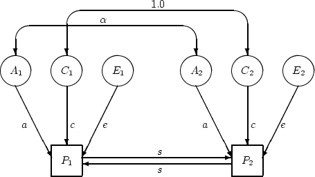
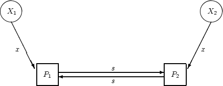
considering the path model in Figure 8.3, which depicts
the influence of an arbitrary latent
Figure 8.3:
Path diagram showing influence
of arbitrary exogenous variable  on phenotype
  in a pair of
relatives (for univariate twin data, incorporating sibling
interaction).
in a pair of
relatives (for univariate twin data, incorporating sibling
interaction).
 |
variable, , on the phenotype . As long as our latent variables
-- A, C, E, etc. -- are independent of each other, their effects
can be considered one at a time and then summed, even in the presence
of social interactions. The linear model corresponding to this path
diagram is
Or, in matrices:
which in turn we can write more economically as
Following the rules for matrix algebra set out in
Chapters 4 and ![[*]](crossref.png) , we can rearrange this
equation, as before:
, we can rearrange this
equation, as before:
and then, multiplying both sides of this equation by the inverse of
(I - B), we have
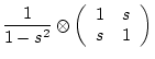
In this case, the matrix (I - B) is simply
which has determinant 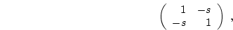 , so
, so
 is
is
The symbol 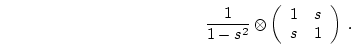 is used to represent the Kronecker product, which
in this case simply means that each element in the matrix is to be
multiplied by the constant
is used to represent the Kronecker product, which
in this case simply means that each element in the matrix is to be
multiplied by the constant
 .
.
We have a vector of phenotypes on the left hand side of
equation 8.8. In the chapter on matrix algebra
(p. ) we showed how the covariance matrix could be
computed from the raw data matrix  by expressing the observed
data as deviations from the mean to form matrix
by expressing the observed
data as deviations from the mean to form matrix  , and computing
the matrix product
, and computing
the matrix product  . The same principle is applied
here to the vector of phenotypes, which has an expected mean of 0 and is thus already expressed in mean deviate form. So to find
the expected variance-covariance matrix of the phenotypes
. The same principle is applied
here to the vector of phenotypes, which has an expected mean of 0 and is thus already expressed in mean deviate form. So to find
the expected variance-covariance matrix of the phenotypes  and
and
 , we multiply by the transpose:
Now in the middle of this equation we have the matrix product
 . This is the covariance matrix of the
x variables. For our particular example, we want two
standardized variables,
. This is the covariance matrix of the
x variables. For our particular example, we want two
standardized variables,  and to have unit variance and
correlation
and to have unit variance and
correlation  so the matrix is:
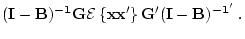
We now have all the pieces required to compute the covariance matrix,
recalling that for this case,
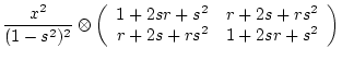
The reader may wish to show as an exercise that by substituting the
right hand sides of equations 8.11 to 8.13
into equation , and carrying out the multiplication,
we obtain:
We can use this result to derive the effects of sibling interaction on
the variance and covariance due to a variety of sources of individual
differences. For example, when considering:
- additive genetic influences,
 and
and  , where
 is 1.0 for MZ twins and 0.5 for DZ twins;
- shared environment influences,
 and
and  ;
;
- non-shared environmental influences,
 and
and  ;
;
- genetic dominance,
 and
and  , where
  for MZ twins and
  for DZ twins.
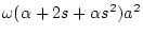
These results are summarized in Table 8.3.
Table 8.3:
The effects of sibling interaction(s) on variance and
covariance components between pairs of relatives.
| Source |
Variance |
Covariance |
| Additive genetic |
 |
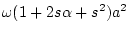 |
| Dominance genetic |
 |
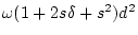 |
| Shared environment |
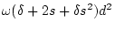 |
|
| Non-shared environment |
 |
 |
 represents the scalar represents the scalar
 obtained from equation 8.14. obtained from equation 8.14. |
Next: 2 Numerical Illustration
Up: 5 Consequences for Variation
Previous: 5 Consequences for Variation
Index
Jeff Lessem
2000-03-20