2 Model-fitting Results

In Table 9.2, we provide selected results from fitting the following models: general sex-limitation (I); common effects sex-limitation (II-IV); and scalar sex-limitation (V). We first note that the general sex-limitation model provides a good fit to the data, with $p=0.32$. The estimate of $a'_{m}$ under this model is fairly small, and when set to zero in model II, found to be non-significant ($\chi^{2}_{1}$ = 2.54, $p > 0.05$). Thus, there is no evidence for sex-specific additive genetic effects, and the common effects sex-limitation model (model II) is favored over the general model. As an exercise, the reader may wish to verify that the same conclusion is reached if the general sex-limitation model with sex-specific dominant genetic effects is compared to the common effects model with $d'_{m}$ removed.

Note that under model II the dominant genetic parameter for females is quite small; thus, when this parameter is fixed to zero in model III, there is not a significant worsening of fit, and model III becomes the most favored model. In model IV, we consider whether the dominant genetic effect for males can also be fixed to zero. The goodness-of-fit statistics indicate that this model fits the data poorly ($p < 0.01$) and provides a significantly worse fit than model III ($\chi^{2}_{1}$ = 26.73, $p < 0.01$). Model IV is therefore rejected and model III remains the favored one.

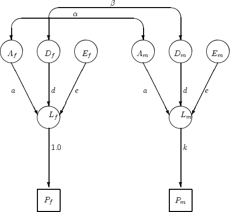
Finally, we consider the scalar sex-limitation model. Since there is evidence for dominant genetic effects in males and not in females, it seems unlikely that this model, which constrains the variance components of females to be scalar multiples of the male variance components, will provide a good fit to the data, unless the additive genetic variance in females is also much smaller than the male additive genetic variance. The model-fitting results support this contention: the model provides a marginal fit to the data ( = 0.05), and is significantly worse than model II ($\chi^2_{2}$ = 7.82, $p < 0.05$ ). We thus conclude from Table 9.2 that III is the best fitting model. This conclusion would also be reached if AIC was used to assess goodness-of-fit.

Table 9.2: Parameter estimates obtained by fitting genotype $\times$ sex interaction models to Virginia and AARP body mass index (BMI) twin data.

	MODEL
Parameter	I	II	III	IV	V
$a_{f}$	0.449	0.454	0.454	0.454	0.346
$d_{f}$	0.172	0.000	-	-	0.288
$e_{f}$	0.264	0.265	0.265	0.267	0.267
$a_{m}$	0.210	0.240	0.240	0.342	-
$d_{m}$	0.184	0.245	0.245	-	-
$e_{m}$	0.213	0.213	0.213	0.220	-
$a'_{m}$	0.198	-	-	-	-
$k$	-	-	-	-	0.778
$\chi^{2}$	9.26	11.80	11.80	38.53	19.62
$d.f.$	8	9	10	11	11
	0.32	0.23	0.30	0.00	0.05
$AIC$	-6.74	-6.20	-8.20	16.53	-2.38

Using the parameter estimates under model III, the expected variance of log BMI (residuals) in males and females can be calculated. A little arithmetic reveals that the phenotypic variance of males is markedly lower than that of females (0.17 vs. 0.28). Inspection of the parameter estimates indicates that the sex difference in phenotypic variance is due to increased genetic and environmental variance in females. However, the increase in genetic variance in females is proportionately greater than the increase in environmental variance, and this difference results in a somewhat larger broad sense (i.e., $a^2+d^2$) heritability estimate for females (75%) than for males (69%).