


Next: 3 Genotype Environment Interaction
Up: 2 Sex-limitation Models
Previous: 2 Scalar Effects Sex-limitation
Index
4 Application to Body Mass Index
In this section, we apply sex-limitation models to data on body mass
index collected from twins in the Virginia Twin Registry and
twins ascertained through the American Association of Retired Persons
(AARP). Details of the membership of these two twin cohorts
are provided in Eaves et al. (1991),
in their analysis of BMI in extended twin-family
pedigrees. In brief, the Virginia twins are members of a population
based registry comprised of 7,458 individuals (Corey et al.,
1986), while the AARP twins are members of a
volunteer registry of 12,118 individuals responding to advertisements
in publications of the AARP. The Virginia twins' mean age is 39.7
years (SD = 14.3), compared to 54.5 years (SD = 16.8) for the AARP
twins. Between 1985 and 1987, Health and Lifestyle questionnaires
were mailed to twins from both of these cohorts. Among the items on
the questionnaire were those pertaining to physical similarity and
confusion in recognition by others (used to diagnose zygosity) and
those asking about current height and weight (used to compute body
mass index). Questionnaires with no missing values for any of these
items were returned by 5,465 Virginia and AARP twin pairs.
From height and weight data, body mass index (BMI) was calculated
for the twins, using the formula:
The natural logarithm of BMI was then taken to normalize the data.
Before calculating covariance matrices of log BMI, the data from the
two cohorts were combined, and the effects of age, age squared, sample
(AARP vs. Virginia), sex, and their interactions were removed. The
resulting covariance matrices are provided in the Mx scripts in
Appendices ![[*]](crossref.png) and , while the
correlations and sample sizes appear in Table 9.1 below.
and , while the
correlations and sample sizes appear in Table 9.1 below.
Table 9.1:
Sample sizes and correlations for BMI data in Virginia
and AARP twins.
| |
|
|
| Zygosity Group |
N |
r |
| MZF |
1802 |
0.744 |
| DZF |
1142 |
0.352 |
| MZM |
750 |
0.700 |
| DZM |
553 |
0.309 |
| DZO |
1341 |
0.251 |
We note that both like-sex MZ correlations are greater than twice the
respective DZ correlations; thus, models with dominant genetic
effects, rather than common environmental effects, were fit to the
data.
In Table 9.2, we provide selected results from fitting the
following models: general sex-limitation (I); common effects
sex-limitation (II-IV); and scalar sex-limitation (V). We first note
that the general sex-limitation model provides a good fit to the data,
with  . The estimate of
 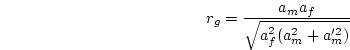 under this model is fairly
small, and when set to zero in model II, found to be non-significant
(
under this model is fairly
small, and when set to zero in model II, found to be non-significant
( = 2.54,
  ). Thus, there is no evidence for
sex-specific additive genetic effects, and the common effects
sex-limitation model (model II) is favored over the general model. As
an exercise, the reader may wish to verify that the same conclusion is
reached if the general sex-limitation model with sex-specific dominant
genetic effects is compared to the common effects model with
). Thus, there is no evidence for
sex-specific additive genetic effects, and the common effects
sex-limitation model (model II) is favored over the general model. As
an exercise, the reader may wish to verify that the same conclusion is
reached if the general sex-limitation model with sex-specific dominant
genetic effects is compared to the common effects model with  removed.
Note that under model II the dominant genetic parameter for females is
quite small; thus, when this parameter is fixed to zero in model III,
there is not a significant worsening of fit, and model III becomes the
most favored model. In model IV, we consider whether the dominant
genetic effect for males can also be fixed to zero. The
goodness-of-fit statistics indicate that this model fits the data
poorly (
removed.
Note that under model II the dominant genetic parameter for females is
quite small; thus, when this parameter is fixed to zero in model III,
there is not a significant worsening of fit, and model III becomes the
most favored model. In model IV, we consider whether the dominant
genetic effect for males can also be fixed to zero. The
goodness-of-fit statistics indicate that this model fits the data
poorly ( ) and provides a significantly worse fit than model
III ( = 26.73, ). Model IV is therefore
rejected and model III remains the favored one.
Finally, we consider the scalar sex-limitation model. Since there is
evidence for dominant genetic effects in males and not in females, it
seems unlikely that this model, which constrains the variance
components of females to be scalar multiples of the male variance
components, will provide a good fit to the data, unless the additive
genetic variance in females is also much smaller than the male
additive genetic variance. The model-fitting results support this
contention: the model provides a marginal fit to the data (
) and provides a significantly worse fit than model
III ( = 26.73, ). Model IV is therefore
rejected and model III remains the favored one.
Finally, we consider the scalar sex-limitation model. Since there is
evidence for dominant genetic effects in males and not in females, it
seems unlikely that this model, which constrains the variance
components of females to be scalar multiples of the male variance
components, will provide a good fit to the data, unless the additive
genetic variance in females is also much smaller than the male
additive genetic variance. The model-fitting results support this
contention: the model provides a marginal fit to the data ( =
0.05), and is significantly worse than model II (
=
0.05), and is significantly worse than model II ( = 7.82,
 ). We thus conclude from Table 9.2 that III is
the best fitting model. This conclusion would also be reached if AIC
was used to assess goodness-of-fit.
). We thus conclude from Table 9.2 that III is
the best fitting model. This conclusion would also be reached if AIC
was used to assess goodness-of-fit.
Table 9.2:
Parameter estimates from fitting genotype  sex
interaction models to BMI.
sex
interaction models to BMI.
| |
|
|
|
|
|
| |
MODEL |
| Parameter |
I |
II |
III |
IV |
V |
 |
0.449 |
0.454 |
0.454 |
0.454 |
0.346 |
 |
0.172 |
0.000 |
- |
- |
0.288 |
 |
0.264 |
0.265 |
0.265 |
0.267 |
0.267 |
 |
0.210 |
0.240 |
0.240 |
0.342 |
- |
 |
0.184 |
0.245 |
0.245 |
- |
- |
 |
0.213 |
0.213 |
0.213 |
0.220 |
- |
|
0.198 |
- |
- |
- |
- |
 |
- |
- |
- |
- |
0.778 |
 |
9.26 |
11.80 |
11.80 |
38.53 |
19.62 |
 |
8 |
9 |
10 |
11 |
11 |
|
0.32 |
0.23 |
0.30 |
0.00 |
0.05 |
 |
-6.74 |
-6.20 |
-8.20 |
16.53 |
-2.38 |
Using the parameter estimates under model III, the expected variance
of log BMI (residuals) in males and females can be calculated. A
little arithmetic reveals that the phenotypic variance of males is
markedly lower than that of females (0.17 vs. 0.28). Inspection of
the parameter estimates indicates that the sex difference in
phenotypic variance is due to increased genetic and
environmental variance in females. However, the increase in
genetic variance in females is proportionately greater than the
increase in environmental variance, and this difference results in a
somewhat larger broad sense (i.e.,  ) heritability estimate
for females (75%) than for males (69%).
The detection of sex-differences in environmental and genetic effects
on BMI leads to questions regarding the nature of these differences.
Speculation might suggest that the somewhat lower male heritability
estimate may be due to the fact that males are less accurate in their
self-report of height and weight than are females. With additional
information, such as test-retest data, this hypothesis could be
rigorously tested. The sex-dependency of genetic dominance is
similarly curious. It may be that the common environment in females
exerts a greater influence on BMI than in males, and, consequently,
masks a genetic dominance effect. Alternatively, the genetic
architecture may indeed be different across the sexes, resulting from
sex differences in selective pressures during human evolution. Again,
additional data, such as that from reared together adopted siblings,
could be used to explore these alternative hypotheses.
One sex-limitation model that we have not considered, but which is
biologically reasonable, is that the across-sex correlation between
additive genetic effects is the same as the across-sex correlation
between the dominance genetic effects
) heritability estimate
for females (75%) than for males (69%).
The detection of sex-differences in environmental and genetic effects
on BMI leads to questions regarding the nature of these differences.
Speculation might suggest that the somewhat lower male heritability
estimate may be due to the fact that males are less accurate in their
self-report of height and weight than are females. With additional
information, such as test-retest data, this hypothesis could be
rigorously tested. The sex-dependency of genetic dominance is
similarly curious. It may be that the common environment in females
exerts a greater influence on BMI than in males, and, consequently,
masks a genetic dominance effect. Alternatively, the genetic
architecture may indeed be different across the sexes, resulting from
sex differences in selective pressures during human evolution. Again,
additional data, such as that from reared together adopted siblings,
could be used to explore these alternative hypotheses.
One sex-limitation model that we have not considered, but which is
biologically reasonable, is that the across-sex correlation between
additive genetic effects is the same as the across-sex correlation
between the dominance genetic effects![[*]](footnote.png) .
Fitting a model of this type involves a non-linear constraint which
can easily be specified in Mx.
.
Fitting a model of this type involves a non-linear constraint which
can easily be specified in Mx.
Next: 3 Genotype Environment Interaction
Up: 2 Sex-limitation Models
Previous: 2 Scalar Effects Sex-limitation
Index
Jeff Lessem
2002-03-21