


Next: 3 Fitting a Phenotypic
Up: 2 Phenotypic Factor Analysis
Previous: 1 Exploratory and Confirmatory
Index
The factor model may be written as
with
and where the measured variables  are a function of a subject's
value on the underlying factor
are a function of a subject's
value on the underlying factor  (henceforth the
  subscript
indicating subjects in will be omitted). These subject values
are called factor scores.
Although the use of factor scores is always implicit in the
application of factor analysis, they cannot be determined precisely
but must be estimated, since the number of common and unique factors
always exceeds the number of observed variables. In addition, there
is a specific part (
subscript
indicating subjects in will be omitted). These subject values
are called factor scores.
Although the use of factor scores is always implicit in the
application of factor analysis, they cannot be determined precisely
but must be estimated, since the number of common and unique factors
always exceeds the number of observed variables. In addition, there
is a specific part ( ) to each variable. The
 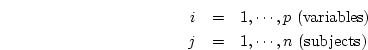 's are the
 -variate factor loadings of measured variables on the latent
factors. To estimate these loadings we do not need to know the
individual factor scores, as the expectation for the
-variate factor loadings of measured variables on the latent
factors. To estimate these loadings we do not need to know the
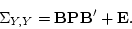
individual factor scores, as the expectation for the  covariance matrix (
 ) consists only of a
  matrix
of factor loadings (B) (
matrix
of factor loadings (B) ( equals
the number of latent factors), a
equals
the number of latent factors), a  correlation matrix of factor scores (P), and a diagonal
matrix of specific variances (E) :
correlation matrix of factor scores (P), and a diagonal
matrix of specific variances (E) :
 |
(59) |
In problems with uncorrelated latent factors, P is an identity
matrix, so equation 10.1 reduces to
 |
(60) |
Thus, the parameters in the model consist of factor loadings and
specific variances (sometimes also referred to as error
variances).
Next: 3 Fitting a Phenotypic
Up: 2 Phenotypic Factor Analysis
Previous: 1 Exploratory and Confirmatory
Index
Jeff Lessem
2002-03-21