


Next: 2 Alternate Representation of
Up: 3 Simple Genetic Factor
Previous: 3 Simple Genetic Factor
Index
1 Multivariate Genetic Factor Model
Using genetic notation, the genetic factor model can be represented as
with
The measured phenotype ( ) (again, omitting the
  subscript)
consists of multiple variables that are a function of a subject's
underlying additive genetic deviate (
subscript)
consists of multiple variables that are a function of a subject's
underlying additive genetic deviate ( ), common (between-families)
environment (
), common (between-families)
environment ( ), and non-shared (within-families) environment (
 ).
In addition, each variable
).
In addition, each variable  has a specific component
  that
itself may consist of a genetic and a non-genetic part. In this
initial application, we assume that is entirely random
environmental in origin, an assumption we relax later. Parameters
that
itself may consist of a genetic and a non-genetic part. In this
initial application, we assume that is entirely random
environmental in origin, an assumption we relax later. Parameters
 ,
,  , and
, and  are the
  -variate factor loadings of measured
variables on the latent factors. A path diagram of this model is shown
in Figure
-variate factor loadings of measured
variables on the latent factors. A path diagram of this model is shown
in Figure ![[*]](crossref.png) .
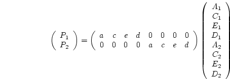
In Mx, there are a number of alternative ways to specify the model.
One approach is to specify the factor structure for the genetic,
shared and specific environmental factors in one matrix, e.g. B
with twice the number of variables (for both twins) as rows and the
number of factors for each twin as columns. If we assume one genetic,
one shared environmental and one specific environmental common factor
per twin
.
In Mx, there are a number of alternative ways to specify the model.
One approach is to specify the factor structure for the genetic,
shared and specific environmental factors in one matrix, e.g. B
with twice the number of variables (for both twins) as rows and the
number of factors for each twin as columns. If we assume one genetic,
one shared environmental and one specific environmental common factor
per twin
 for our four-variate
arithmetic computation example (shown as T0 - T3 to represent
administration times 0-3 before and after standard doses of alcohol
for twin 1 (Tw1) and twin 2 (Tw2) respectively), the B matrix
would look like
for our four-variate
arithmetic computation example (shown as T0 - T3 to represent
administration times 0-3 before and after standard doses of alcohol
for twin 1 (Tw1) and twin 2 (Tw2) respectively), the B matrix
would look like
In this case with 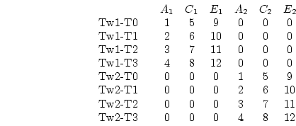 factors and four observed variables for each
twin (p=8), B would be a
factors and four observed variables for each
twin (p=8), B would be a  (
( ) matrix of the
factor loadings, P the
) matrix of the
factor loadings, P the  correlation matrix of factor
scores, and E a
correlation matrix of factor
scores, and E a  diagonal matrix of unique
variances. The
expected covariance may then be calculated as in
equation 10.1:
diagonal matrix of unique
variances. The
expected covariance may then be calculated as in
equation 10.1:
 |
(61) |
In a multivariate analysis of twin data according to this factor model,
 is a
is a  predicted covariance matrix of observations on
twin 1 and twin 2 and B is a
predicted covariance matrix of observations on
twin 1 and twin 2 and B is a  matrix of loadings of
these observations on latent genotypes and non-shared and common
environments of twin 1 and twin 2. The factor loadings between
matrix of loadings of
these observations on latent genotypes and non-shared and common
environments of twin 1 and twin 2. The factor loadings between  and
and
 ,
,  and
and  , and
, and  and
and  are constrained to be equal
for twin 1 and twin 2, similar to the path coefficients of the univariate
models discussed in previous chapters. The equality constraints on the
parameters are obtained in Mx by using the same non-zero parameter number
in a
are constrained to be equal
for twin 1 and twin 2, similar to the path coefficients of the univariate
models discussed in previous chapters. The equality constraints on the
parameters are obtained in Mx by using the same non-zero parameter number
in a Specification statement for the free parameters. The unique
variances also are equal for both members of a twin pair. These may be
estimated on the diagonal of the E matrix (e.g.,
Heath et al., 1989c). To fit
this model, B and E are estimated from the data and P
( ) must be fixed a priori (for example, the correlation
between for twin 1 and for twin 2 is 1.0 for MZ and 0.5 for DZ
twins; the correlation between the variables of twin 1 and twin 2 is
1.0).
One alternative specification of this model is to include the unique
variances in matrix B and fix E to zero. The factor patterns
for and of twin 1 and twin 2 are identical to that in
Section 10.2.3. The main difference lies in the treatment of the
unique variances. In the earlier example these were estimated as
variances on the diagonal of E, but now they are modeled as the
square roots of the variances. These quantities are now square roots
because the unique variances are calculated as the product
) must be fixed a priori (for example, the correlation
between for twin 1 and for twin 2 is 1.0 for MZ and 0.5 for DZ
twins; the correlation between the variables of twin 1 and twin 2 is
1.0).
One alternative specification of this model is to include the unique
variances in matrix B and fix E to zero. The factor patterns
for and of twin 1 and twin 2 are identical to that in
Section 10.2.3. The main difference lies in the treatment of the
unique variances. In the earlier example these were estimated as
variances on the diagonal of E, but now they are modeled as the
square roots of the variances. These quantities are now square roots
because the unique variances are calculated as the product
 in the expected covariance expression whereas in the previous
example the quantities were estimated as the unproducted quantity E.
One might expect that this subtle change would have no effect on the model
(as indeed it does not in this example), but on occasion these alternative
residual specifications may produce different outcomes. The situation of
residual variances
in the expected covariance expression whereas in the previous
example the quantities were estimated as the unproducted quantity E.
One might expect that this subtle change would have no effect on the model
(as indeed it does not in this example), but on occasion these alternative
residual specifications may produce different outcomes. The situation of
residual variances  makes little sense in genetic analyses because
it implies an impossible negative variance component. Consequently,
although it may be possible to make alternative representations like this
in Mx, we recommend this model, as it constrains unique variances to be
makes little sense in genetic analyses because
it implies an impossible negative variance component. Consequently,
although it may be possible to make alternative representations like this
in Mx, we recommend this model, as it constrains unique variances to be
 . Nevertheless, both methods give identical solutions when
fitted to the data used in these examples.
. Nevertheless, both methods give identical solutions when
fitted to the data used in these examples.
Next: 2 Alternate Representation of
Up: 3 Simple Genetic Factor
Previous: 3 Simple Genetic Factor
Index
Jeff Lessem
2002-03-21