


Next: 4 Fitting a Second
Up: 3 Simple Genetic Factor
Previous: 2 Alternate Representation of
Index
3 Fitting the Multivariate Genetic Model
To illustrate the genetic common factor model we fit it to the
arithmetic computation data, but now using both members of the female
twin pairs and specifying two groups for the MZ and DZ twins. The
observed variances and correlations examined in this analysis are
presented in Table 10.3. Appendix ![[*]](crossref.png) shows
the full Mx script for this model.
shows
the full Mx script for this model.
Table 10.3:
Observed female MZ (above diagonal) and DZ (below diagonal)
correlations and variances for arithmetic computation variables.
| |
|
Twin 1 |
Twin 2 |
| |
|
T0 |
T1 |
T2 |
T3 |
T0 |
T1 |
T2 |
T3 |
| T1 |
T0 |
1.0 |
.81 |
.83 |
.87 |
.78 |
.65 |
.71 |
.68 |
| |
T1 |
.89 |
1.0 |
.87 |
.87 |
.74 |
.74 |
.74 |
.71 |
| |
T2 |
.85 |
.90 |
1.0 |
.90 |
.73 |
.66 |
.72 |
.70 |
| |
T3 |
.83 |
.86 |
.86 |
1.0 |
.74 |
.71 |
.74 |
.75 |
| T2 |
T0 |
.23 |
.31 |
.36 |
.34 |
1.0 |
.73 |
.78 |
.79 |
| |
T1 |
.22 |
.32 |
.34 |
.38 |
.81 |
1.0 |
.86 |
.87 |
| |
T2 |
.16 |
.23 |
.27 |
.35 |
.79 |
.86 |
1.0 |
.87 |
| |
T3 |
.23 |
.31 |
.34 |
.37 |
.81 |
.86 |
.87 |
1.0 |
| |
MZ |
297.9 |
229.4 |
247.4 |
274.9 |
281.9 |
359.7 |
326.9 |
281.1 |
| |
DZ |
259.7 |
259.9 |
245.2 |
249.3 |
283.8 |
249.5 |
262.1 |
270.9 |
The results from this common factor model are shown in Table 10.3.3
The parameter estimates in the MX PARAMETER ESTIMATES section
indicate a substantial genetic basis for the observed arithmetic
covariances, as the genetic loadings are much higher than either the
shared and non-shared environmental effects. The unique variances in
F also appear substantial but these do not contribute to
covariances among the measures, only to the variance of each observed
variable. The  value of 46.77 suggests that this single
factor model provides a reasonable explanation of the data. (Note that
the 56 degrees of freedom are obtained from
value of 46.77 suggests that this single
factor model provides a reasonable explanation of the data. (Note that
the 56 degrees of freedom are obtained from
 free
statistics minus 16 estimated parameters).
free
statistics minus 16 estimated parameters).
Table 10.4:
Parameter estimates from the full genetic common factor model
| |
|
|
|
|
| |
 |
 |
 |
 |
| Time 1 |
15.088 |
1.189 |
4.142 |
46.208 |
| Time 2 |
13.416 |
5.119 |
6.250 |
39.171 |
| Time 3 |
13.293 |
4.546 |
7.146 |
31.522 |
| Time 4 |
13.553 |
5.230 |
5.765 |
34.684 |
 , 56 df, p=.806 , 56 df, p=.806 |
Earlier in this chapter we alluded to the fact that confirmatory factor
models allow one to statistically test the significance of model parameters. We can perform such a test on the present
multivariate genetic model. The Mx output above shows that the shared
environment factor loadings are much smaller than either the genetic or
non-shared environment loadings. We can test whether these loadings are
significantly different from zero by modifying slightly the Mx script to
fix these parameters and then re-estimating the other model parameters.
There are several possible ways in which one might modify the script to
accomplish this task, but one of the easiest methods is simply to change
the Y to have no free elements.
Performing this modification in the first group effectively drops all  loadings from all groups because the
 Matrices= Group 1 statement in
the second and third group equates its loadings to those in the first.
Thus, the modified script represents a model in which common factors are
hypothesized for genetic and non-shared environmental effects to account
for covariances among the observed variables, and unique effects are
allowed to contribute to measurement variances. All shared environmental
effects are omitted from the model.
Since the modified multivariate model is a sub- or nested model of
the full common factor specification, comparison of the goodness-of-fit
chi-squared values provides a test of the significance of the deleted
factor loadings (see Chapter ). The full model has 56 degrees
of freedom and the reduced one:
 d.f. Thus,
the difference chi-squared statistic for the test of loadings has
d.f. Thus,
the difference chi-squared statistic for the test of loadings has  degrees of freedom. As may be seen in the output fragment
below, the
degrees of freedom. As may be seen in the output fragment
below, the  of the reduced model is 51.08, and, therefore,
the difference
of the reduced model is 51.08, and, therefore,
the difference  is
is
 , which is
non-significant at the .05 level. This non-significant chi-squared
indicates that the shared environmental loadings can be dropped from the
multivariate genetic model without significant loss of fit; that is, the
arithmetic data are not influenced by environmental effects shared by
twins. Parameter estimates from this reduced model are given below in
Table 10.3.3
, which is
non-significant at the .05 level. This non-significant chi-squared
indicates that the shared environmental loadings can be dropped from the
multivariate genetic model without significant loss of fit; that is, the
arithmetic data are not influenced by environmental effects shared by
twins. Parameter estimates from this reduced model are given below in
Table 10.3.3
Table 10.5:
Parameter estimates from the reduced genetic common factor model
| |
|
|
|
|
| |
|
|
|
|
| Time 1 |
14.756 |
 |
3.559 |
59.502 |
| Time 2 |
14.274 |
|
6.331 |
39.433 |
| Time 3 |
14.081 |
|
7.047 |
30.843 |
| Time 4 |
14.405 |
|
5.845 |
36.057 |
 , 60 df, p=.787 , 60 df, p=.787 |
The estimates for the genetic and non-shared environment parameters differ
somewhat between the reduced model and those estimated in the full common
factor model. Such differences often appear when fitting nested models,
and are not necessarily indicative of misspecification (of course, one
would not expect the estimates to change in the case where parameters to
be omitted are estimated as 0.0 in the full model). The fitting functions
used in Mx (see Chapter ) are designed to produce parameter
estimates that yield the closest match between the observed and estimated
covariance matrices. Omission of selected parameters, for example, the
loadings in the present model, generates a different model 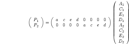 and thus may be expected to yield slightly different parameter estimates
in order to best approximate the observed matrix.
and thus may be expected to yield slightly different parameter estimates
in order to best approximate the observed matrix.
Next: 4 Fitting a Second
Up: 3 Simple Genetic Factor
Previous: 2 Alternate Representation of
Index
Jeff Lessem
2002-03-21