1 Genetic and Environmental Correlations

We now turn from the one- and two-factor multivariate genetic models described above and consider more general multivariate formulations which may encompass many genetic and environmental factors. These more general approaches subsume the simpler techniques described above. Consider a simple extension of the one- and two-factor AE models for multiple variables (sections 10.3.2-10.3.4). The total phenotypic covariance matrix in a population, ${\bf C_p}$, can be decomposed into an additive genetic component, A, and a random environmental component, E:

$${\bf C_p} = {\bf A} + {\bf E}\; ,$$ (62)

We are leaving out the shared environment in this example just for simplicity. More complex expectations for 10.4 may be written without affecting the basic idea. ``A'' is called the additive genetic covariance matrix and ``E'' the random environmental covariance matrix. If A is diagonal, then the traits comprising A are genetically independent; that is, there is no ``additive genetic covariance'' between them. One interpretation of this is that different genes affect each of the traits. Similarly, if the environmental covariance matrix, E, is diagonal, we would conclude that each trait is affected by quite different environmental factors. On the other hand, suppose A were to have significant off-diagonal elements. What would that mean? Although there are many reasons why this might happen, one possibility is that at least some genes are having effects on more than one variable. This is known as pleiotropy in the classical genetic literature (see Chapter 3). Similarly, significant off-diagonal elements in E (or C, if it were included in the model) would indicate that some environmental factors influence more than one trait at a time. 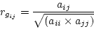The extent to which the same genes or environmental factors contribute to the observed phenotypic correlation between two variables is often measured by the genetic or environmental correlation between the variables. If we have estimates of the genetic and environmental covariance matrices, A and E, the genetic correlation ($r_g$) between variables $i$ and $j$ is

$$r_{g_{ij}} = \frac{a_{ij}}{\sqrt{(a_{ii} \times a_{jj})}}$$ (63)

and the environmental correlation, similarly, is

$$r_{e_{ij}} = \frac{e_{ij}}{\sqrt{(e_{ii} \times e_{jj})}} \; .$$ (64)

The analogy with the familiar formula for the correlation coefficient is clear. The genetic covariance between two phenotypes is quite distinct from the genetic correlation. It is possible for two traits to have a very high genetic correlation yet have little genetic covariance. Low genetic covariance could arise if either trait had low genetic variance. Vogler (1982) and Carey (1988) discuss these issues in greater depth.