Next: 2 Using SAS or
Up: 2 Continuous Data Analysis
Previous: 2 Continuous Data Analysis
Index
1 Calculating Summary Statistics by Hand
The variances and covariances used in twin analyses often are computed using a
statistical package such as SPSS [SPSS, 1988] or SAS [SAS, 1988], or by PRELIS
[]. Nevertheless, it is
useful to examine how they are
calculated in order to ensure a comprehensive understanding of one's observed
data. In this section we describe the calculation of means, variances,
covariances, and correlations.
Some simulated measurements from 16 MZ and 16 DZ twin pairs are presented in
Table 2.1. The observed values in the columns labelled
Twin 1
Table 2.1:
Simulated measurements from 16 MZ and 16 DZ Twin Pairs.
| |
|
|
|
| MZ |
DZ |
| Twin 1 |
Twin 2 |
Twin 1 |
Twin 2 |
| 3 |
2 |
0 |
1 |
| 3 |
3 |
2 |
3 |
| 2 |
1 |
1 |
2 |
| 1 |
2 |
4 |
3 |
| 0 |
0 |
3 |
1 |
| 2 |
2 |
2 |
2 |
| 2 |
2 |
2 |
2 |
| 3 |
2 |
1 |
3 |
| 3 |
3 |
3 |
4 |
| 2 |
3 |
1 |
0 |
| 1 |
1 |
1 |
1 |
| 1 |
1 |
2 |
1 |
| 4 |
4 |
3 |
3 |
| 2 |
3 |
3 |
2 |
| 2 |
1 |
2 |
2 |
| 1 |
2 |
2 |
2 |
and Twin 2 have been selected to illustrate some elementary
principles of variation in twins![[*]](footnote.png) .
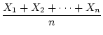
In order to obtain the summary statistics of variances and covariances
for genetic analysis, it is first necessary to compute the average
value for a set of measurements, called the
mean.
The mean is typically denoted by a bar over the variable name for a
group of observations, for example
.
In order to obtain the summary statistics of variances and covariances
for genetic analysis, it is first necessary to compute the average
value for a set of measurements, called the
mean.
The mean is typically denoted by a bar over the variable name for a
group of observations, for example  or
or
 or
or
 . The formula for calculation of the mean
is:
. The formula for calculation of the mean
is:
in which 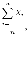 represents the
  observation and
  is the
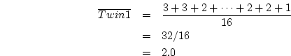
total number of observations. In the twin data of
Table 2.1, the mean of the measurements on Twin 1 of the
MZ pairs is
is the
total number of observations. In the twin data of
Table 2.1, the mean of the measurements on Twin 1 of the
MZ pairs is
The mean for the second MZ twin (
) also is 2.0, as are the means for both DZ twins.
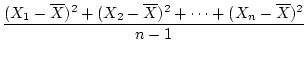
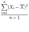
The variance of the observations represents a
measure of dispersion
around the mean; that is, how much, on average, observations differ from the
mean. The variance formula for a sample of measurements, often represented as
 or
or  or
or  , is
, is
We note two things:
first, the difference between each observation and the mean is squared. In
principle, absolute differences from the mean could be used as a measure of
variation, but absolute differences have a greater variance than squared
differences [Fisher, 1920], and are therefore less efficient for use as a
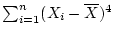
summary statistic. Likewise, higher powers (e.g.
 ) also have greater variance. In fact, Fisher showed that
the square of the difference
is the most informative measure of variance, i.e., it is a sufficient
statistic. Second, the sum of the
squared deviations is divided by
) also have greater variance. In fact, Fisher showed that
the square of the difference
is the most informative measure of variance, i.e., it is a sufficient
statistic. Second, the sum of the
squared deviations is divided by
 rather than . The denominator is in order to compensate for
an underestimate in the sample variance which would be obtained if were
divided by . (This arises from the fact that we have already used one
parameter -- the mean -- to describe the data; see Mood & Graybill, 1963
for a discussion of bias in sample
variance). Again using the twin data in Table 2.1
as an example, the variance of MZ Twin 1 is
rather than . The denominator is in order to compensate for
an underestimate in the sample variance which would be obtained if were
divided by . (This arises from the fact that we have already used one
parameter -- the mean -- to describe the data; see Mood & Graybill, 1963
for a discussion of bias in sample
variance). Again using the twin data in Table 2.1
as an example, the variance of MZ Twin 1 is
The variances of data from the second MZ twin, DZ Twin 1, and DZ Twin
2 also equal 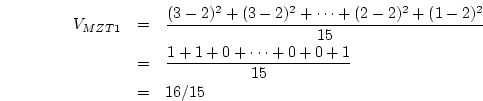 .
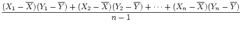
Covariances
are computationally similar to
variances, but represent
mean deviations which are shared by two sets of observations. In the
twin example, covariances are useful because they indicate the extent
to which deviations from the mean by Twin 1 are similar to the second
twin's deviations from the mean. Thus, the covariance between
observations of Twin 1 and Twin 2 represents a scale-dependent measure
of twin similarity. Covariances are often denoted by
.
Covariances
are computationally similar to
variances, but represent
mean deviations which are shared by two sets of observations. In the
twin example, covariances are useful because they indicate the extent
to which deviations from the mean by Twin 1 are similar to the second
twin's deviations from the mean. Thus, the covariance between
observations of Twin 1 and Twin 2 represents a scale-dependent measure
of twin similarity. Covariances are often denoted by  or Cov
 or Cov
 , and are calculated as
Note that the variance formula shown in Eq. 2.2 is
just a special case of the covariance when 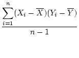 . In other
words, the variance is simply the covariance between a variable and
itself.
For the twin data in Table 2.1, the covariance between
MZ twins is
. In other
words, the variance is simply the covariance between a variable and
itself.
For the twin data in Table 2.1, the covariance between
MZ twins is
The covariance between DZ pairs may be calculated similarly to give
8/15.
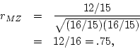
The correlation coefficient
is
closely related to the covariance between two sets of observations.
Correlations may be interpreted in a similar manner as covariances,
but are rescaled to give a lower bound of -1.0 and an upper bound of 1.0.
The correlation coefficient, 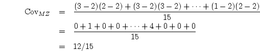 , may be calculated using the
covariance between two measures and the square root of the variance
(the standard deviation)
of each measure:
, may be calculated using the
covariance between two measures and the square root of the variance
(the standard deviation)
of each measure:
 |
(4) |
For the simulated MZ twin data, the correlation between twins is
and the DZ twin correlation is
Although variances and covariances typically define the observed
information for biometrical analyses of twin data, correlations
are useful for comparing resemblances between twins as a function of
genetic relatedness. In the simulated twin data, the MZ twin
correlation (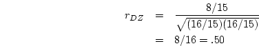 ) is greater than that of the DZ twins (
 ). This greater similarity of MZ twins may be due to several
sources of variation (discussed in subsequent chapters), but at the
least is suggestive of a heritable basis for the trait, as increased
MZ similarity could result from the fact that MZ twins are genetically
identical, whereas DZ twins share only 1/2 of their genes on average.
). This greater similarity of MZ twins may be due to several
sources of variation (discussed in subsequent chapters), but at the
least is suggestive of a heritable basis for the trait, as increased
MZ similarity could result from the fact that MZ twins are genetically
identical, whereas DZ twins share only 1/2 of their genes on average.
Next: 2 Using SAS or
Up: 2 Continuous Data Analysis
Previous: 2 Continuous Data Analysis
Index
Jeff Lessem
2002-03-21