


Next: 2 Variance Components Model:
Up: 6 Path Models for
Previous: 6 Path Models for
Index
1 Path Coefficients Model: Example of Standardized Tracing Rules
When applying the tracing rules, it helps to draw out each tracing
route to ensure that they are neither forgotten nor traced twice. In
the traditional path model of Figure 5.3a, to derive the
expected twin covariance for the case of
monozygotic twin pairs reared together, we can trace the following routes:
so that the expected covariance between MZ twin pairs reared together
will be
 |
(30) |
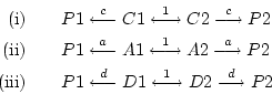
In the case of dizygotic twin pairs reared together, we can trace the following routes:
yielding an expected covariance between DZ twin pairs of
 |
(31) |
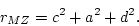
The expected variance of a variable -- again
assuming we are working with standardized variables -- is derived by
tracing all possible routes from the variable back to itself, without
violating any of the tracing rules given in Section 5.4.1
above. Thus, following paths from P1 to itself we have
yielding the predicted variance for 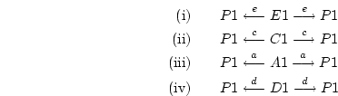 or
or  in Figure 5.3a
of
in Figure 5.3a
of
 |
(32) |
An important assumption implicit in Figure 5.3 is that an
individual's additive genetic deviation is uncorrelated with his or
her shared environmental deviation (i.e., there are no arrows
connecting the latent  and
and  variables of an individual). In
Chapter
variables of an individual). In
Chapter ![[*]](crossref.png) we shall discuss how this assumption can be
relaxed. Also implicit in the coefficient of 0.5 for the covariance
of the additive genetic values of DZ twins or siblings is the
assumption of random mating, which we shall also relax in
Chapter .
we shall discuss how this assumption can be
relaxed. Also implicit in the coefficient of 0.5 for the covariance
of the additive genetic values of DZ twins or siblings is the
assumption of random mating, which we shall also relax in
Chapter .
Next: 2 Variance Components Model:
Up: 6 Path Models for
Previous: 6 Path Models for
Index
Jeff Lessem
2002-03-21