


Next: 1 Path Coefficients Model:
Up: 5 Path Analysis and
Previous: 5 Path Models for
Index
6 Path Models for the Classical Twin Study
To introduce genetic models and to further illustrate the tracing
rules both for standardized variables and unstandardized variables, we
examine some simple genetic models of resemblance. The classical twin
study, in which MZ twins and DZ twins are reared together in the same
home is one of the most powerful designs for detecting genetic and
shared environmental effects. Once we have collected such data, they
may be summarized as observed covariance matrices
(Chapter 2), but in order to test hypotheses we need to
derive expected covariance matrices from the model. We first digress
briefly to review the biometrical principles outlined in
Chapter 3, in order to express the ideas in a
path-analytic context.
In contrast to the regression models considered in previous sections,
many genetic analyses of family data postulate independent variables
(genotypes and environments) as latent rather than manifest
variables. In other words, the genotypes and environments are not
measured directly but their influence is inferred through their
effects on the covariances of relatives. However, we can represent
these models as path diagrams in just the same way as the
regression models. The brief introduction to path-analytic genetic models
we give here will be treated in greater detail in Chapter 6,
and thereafter.
From quantitative genetic theory (see Chapter 3), we can
write equations relating the phenotypes  and
and  of relatives
 and
and  (e.g., systolic blood pressures of first and second
members of a twin pair), to their underlying genotypes and
environments. We may decompose the total genetic effect on a
phenotype into that due to the additive effects of alleles at multiple
loci, that due to the dominance effects at multiple loci, and that due
to the epistatic interactions between loci (Mather and Jinks, 1982).
Similarly, we may decompose the total environmental effect into that
due to environmental influences shared by twins or sibling pairs
reared in the same family (`shared', `common', or `between-family'
environmental effects), and that due to environmental effects which
make family members differ from one another (`random', `specific', or
`within-family' environmental effects). Thus,
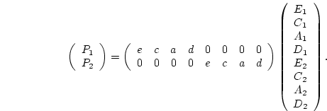
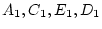
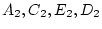
the observed phenotypes, and , are assumed to be linear
functions of the underlying additive genetic variance (
(e.g., systolic blood pressures of first and second
members of a twin pair), to their underlying genotypes and
environments. We may decompose the total genetic effect on a
phenotype into that due to the additive effects of alleles at multiple
loci, that due to the dominance effects at multiple loci, and that due
to the epistatic interactions between loci (Mather and Jinks, 1982).
Similarly, we may decompose the total environmental effect into that
due to environmental influences shared by twins or sibling pairs
reared in the same family (`shared', `common', or `between-family'
environmental effects), and that due to environmental effects which
make family members differ from one another (`random', `specific', or
`within-family' environmental effects). Thus,
the observed phenotypes, and , are assumed to be linear
functions of the underlying additive genetic variance ( and
and
 ), dominance variance (
 and
and  ), shared environmental
variance (
), shared environmental
variance ( and
and  ) and random environmental variance (
 and
and  ). In quantitative genetic studies of human populations,
epistatic genetic effects are usually confounded with dominance
genetic effects, and so will not be considered further here. Assuming
all variables are scaled as deviations from zero, we have
). In quantitative genetic studies of human populations,
epistatic genetic effects are usually confounded with dominance
genetic effects, and so will not be considered further here. Assuming
all variables are scaled as deviations from zero, we have
and
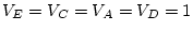
Particularly for pairs of twins, we do not expect the magnitude of
genetic or environmental effects to vary as a function of
relationship![[*]](footnote.png) so we set
so we set  ,
,  ,
,
 , and
, and  . In matrix form, we write
Unless two or more waves of measurement are used, or several
observed variables index the phenotype under study, residual effects
are included in the random environmental component, and are not
separately specified in the model.
Figures 5.3a and 5.3b represent two alternative
parameterizations of the basic genetic model, illustrated for the case
of pairs of monozygotic twins (MZ) or
dizygotic twins (DZ), who may be
reared
together (MZT, DZT) or
reared apart (MZA, DZA). In Figure 5.3a, the
traditional path coefficients model, the variances of the latent
variables
 and
and
 are
standardized (
are
standardized (
 , and the path coefficients
 , or
, or  -- quantifying the paths from the latent variables
to the observed variable, measured on both twins,
-- quantifying the paths from the latent variables
to the observed variable, measured on both twins,  and
and  --
are free parameters to be estimated. Figure 5.3b is called a
variance components model because it fixes
--
are free parameters to be estimated. Figure 5.3b is called a
variance components model because it fixes
 ,
and estimates separate random environmental, shared environmental,
additive genetic and dominance genetic variances instead.
,
and estimates separate random environmental, shared environmental,
additive genetic and dominance genetic variances instead.
Figure 5.3:
Alternative representations of the basic genetic model: a)
traditional path coefficients model, and b) variance components model.
 |
The traditional path model illustrates tracing rules for standardized
variables, and is straightforward to generalize to multivariate
problems; the variance components model illustrates an unstandardized
path model. Provided all parameter estimates are non-negative,
tracing the paths in either parameterization will give the same
solution, with  ,
,  ,
,  and
and  .
.
Subsections
Next: 1 Path Coefficients Model:
Up: 5 Path Analysis and
Previous: 5 Path Models for
Index
Jeff Lessem
2002-03-21