2 Graphing and Quantifying Familial Resemblance

Look at the two sets of data shown in Figure 1.2. The first

Figure 1.2: Two scatterplots of weight in: a) a large sample of DZ twin pairs, and b) pairs of individuals matched at random.

part of the figure is a scatterplot of measurements of weight in a large sample of non-identical (fraternal, dizygotic, DZ) twins. Each cross in the diagram represents a single twin pair. The second part of the figure is a scatterplot of pairs of completely unrelated people from the same population. Notice how the two parts of the figure differ. In the unrelated pairs the pattern of crosses gives the general impression of being circular; in general, if we pick a particular value on the X axis (first person's weight), it makes little difference to how heavy the second person is on average. This is what it means to say that measures are uncorrelated -- knowing the score of the first member of a pair makes it no easier to predict the score of the second and vice-versa. By comparison, the scatterplot for the fraternal twins (who are related biologically to the same degree as brothers and sisters) looks somewhat different. The pattern of crosses is slightly elliptical and tilted upwards. This means that as we move from lighter first twins towards heavier first twins (increasing values on the X axis), there is also a general tendency for the average scores of the second twins (on the Y axis) to increase. It appears that the weights of twins are somewhat correlated. Of course, if we take any particular X value, the Y values are still very variable so the correlation is not perfect. The correlation coefficient (see Chapter 2) allows us to quantify the degree of relationship between the two sets of measures. In the unrelated individuals, the correlation turns out to be 0.02 which is well within the range expected simply by chance alone if the measures were really independent. For the fraternal twins, on the other hand, the correlation is 0.44 which is far greater than we would expect in so large a sample if the pairs of measures were truly independent. The data on weight illustrate the important general point that relatives are usually much more alike than unrelated individuals from the same population. That is, although there are large individual differences for almost every trait than can be measured, we find that the trait values of family members are often quite similar.

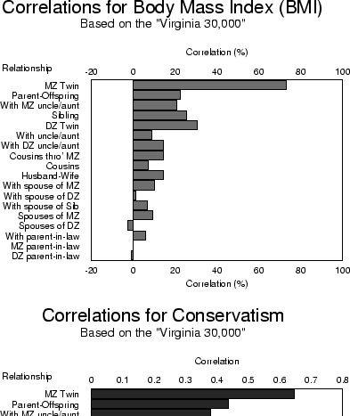
Figure 1.3: Correlations for body mass index (weight/height$^2$) and conservatism between relatives. Data were obtained from large samples of nuclear families ascertained through twins.

Figure 1.3 gives the correlations between relatives in large samples of nuclear families for body mass index (BMI), and conservatism. One simple way of interpreting the correlation coefficient is to multiply it by 100 and treat it as a percentage. The correlation ($\times$ 100) is the ``percentage of the total variation in a trait which is caused by factors shared by members of a pair." Thus, for example, our correlation of 0.44 for the weights of DZ twins implies that, of all the factors which create variation in weight, 44% are factors which members of a DZ twin pair have in common. We can offer a similar interpretation for the other kinds of relationship. A problem becomes immediately apparent. Since the DZ twins, for example, have spent most of their lives together, we cannot know whether the 44% is due entirely to the fact that they shared the same environment in utero, lived with the same parents after birth, or simply have half their genes in common -- and we shall never know until we can find another kind of relationship in which the degree of genetic similarity, or shared environmental similarity, is different. 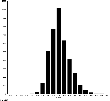Figure 1.4 gives a scattergram for the weights of a large

Figure 1.4: Scatterplot of weight in a large sample of MZ twins.

sample of identical (monozygotic, MZ) twins. Whereas DZ twins, like siblings, on average share only half their genes, MZ twins are genetically identical. The scatter of points is now much more clearly elliptical, and the $45^\circ$ tilt of the major axis is especially obvious. The correlation in the weights in this sample of MZ twins is 0.77, almost twice that found for DZ's. The much greater resemblance of MZ twins, who are expected to have completely identical genes establishes a strong prima facie case for the contribution of genetic factors to differences in weight. One of the tasks to be addressed in this book is how to interpret such differential patterns of family resemblance in a more rigorous, quantitative, fashion.