


Next: 7 Power and Sample
Up: 6 Univariate Analysis
Previous: 1 Major Depressive Disorder
Index
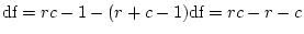
4 Model for Age-Correction of Twin Data
We now turn to a slightly more elaborate example of univariate
analysis, using data from the Australian twin sample that were used in
the BMI example earlier, but in this case data on social
attitudes. Factor analysis of the item responses revealed a major
dimension with low scores indicating radical attitudes and high scores
indicating attitudes commonly labelled as ``conservative.'' Our a priori
expectation is that variation in this dimension will be largely shaped
by social environment and that genetic factors will be of little or no
importance. This expectation is based on the differences between the
MZ and DZ correlations;  and
and  ,
indicating little, if any, genetic influence on social attitudes. We
also might expect that conservatism scores are affected by age. We
can use the Mx script in Appendix
,
indicating little, if any, genetic influence on social attitudes. We
also might expect that conservatism scores are affected by age. We
can use the Mx script in Appendix ![[*]](crossref.png) to examine the age
effects, reading in the age of each twin pair and
the conservatism scores for twin 1 (
to examine the age
effects, reading in the age of each twin pair and
the conservatism scores for twin 1 (Cons_t1) and twin 2
(Cons_t2). Since in this specification we have 3 indicator variables, we adjust
NInput_vars=3. If we initially ignore age, as an exploratory
analysis, we can select only the conservatism scores for analysis,
using the Select command (note that the list of variables
selected must end with a semicolon `;').
The script fits the ACE model. The results of this model
are presented in the fourth line of the standardized results of Table 6.11, which
shows that the squares of parameters estimated from the model sum to
one, because these correspond to the proportions of variance
associated with each source (A, C, and E).
Table 6.11:
Conservatism in Australian females: standardized parameter
estimates for additive genotype (A), common environment (C), random
environment (E) and dominance genotype (D).
| |
Parameter Estimates |
Fit statistics |
| Model |
 |
 |
 |
 |
 |
df |
 |
 |
-- |
-- |
1.000 |
-- |
823.76 |
5 |
.000 |
 |
-- |
0.804 |
0.595 |
-- |
19.41 |
4 |
.001 |
 |
0.836 |
-- |
0.549 |
-- |
56.87 |
4 |
.000 |
 |
0.464 |
0.687 |
0.559 |
-- |
3.07 |
3 |
.380 |
 |
0.836 |
-- |
0.549 |
0.000 |
56.87 |
3 |
.000 |
The significance of common environmental contributions to variance in
conservatism may be tested by dropping (AE model) but this
leads to a worsening of by 53.8 for 1 d.f., confirming its
importance. Similarly, the poor fit of the CE model confirms that
genetic factors also contribute to individual differences
(significance of is
 for 1 df, which is highly
significant). The model, which hypothesizes that there is no
family resemblance for conservatism, is overwhelmingly rejected,
illustrating of the great power of this data set to discriminate
between competing hypotheses. For interest, we also present the
results of the ADE model. Since we have already noted that
for 1 df, which is highly
significant). The model, which hypothesizes that there is no
family resemblance for conservatism, is overwhelmingly rejected,
illustrating of the great power of this data set to discriminate
between competing hypotheses. For interest, we also present the
results of the ADE model. Since we have already noted that  is appreciably greater than half the MZ correlation, it is clear that
this model is inappropriate. Symmetric with the results of fitting an
ACE model to the BMI data (where
is appreciably greater than half the MZ correlation, it is clear that
this model is inappropriate. Symmetric with the results of fitting an
ACE model to the BMI data (where  was still less than
 , indicating dominance), we now find that the estimate of
gets ``stuck" on its lower bound of zero. The BMI and conservatism
examples illustrate in a practical way the perfect reciprocal
dependence of and in the classical twin design of which only
one may be estimated. The issue of the reciprocal confounding of
shared environment and genetic non-additivity (dominance or epistasis)
in the classical twin design has been discussed in detail in papers by
Martin et al., (1978), Grayson (1989),
and Hewitt (1989).
It is clear from the results above that there are major influences of
the shared environment on conservatism. One aspect of the environment
that is shared with perfect correlation by cotwins is their age. If a
variable is strongly related to age and if a twin sample is drawn from
a broad age range, as opposed to a cohort sample covering a narrow
range of birth years, then differences between twin pairs in age will
contribute to estimated common environmental variance. This is the case
for the twins in the Australian sample, who range from 18 to 88 years
old. It is clearly of interest to try to separate this variance due
to age differences from genuine cultural differences contributing to
the estimate of .
Fortunately, structural equation modeling, which is based on linear
regression, provides a very easy way of allowing for the effects of
age regression while simultaneously estimating the genetic and
environmental effects (Neale and
Martin, 1989). Figure 6.2
illustrates the method with a path diagram, in
which the regression of
, indicating dominance), we now find that the estimate of
gets ``stuck" on its lower bound of zero. The BMI and conservatism
examples illustrate in a practical way the perfect reciprocal
dependence of and in the classical twin design of which only
one may be estimated. The issue of the reciprocal confounding of
shared environment and genetic non-additivity (dominance or epistasis)
in the classical twin design has been discussed in detail in papers by
Martin et al., (1978), Grayson (1989),
and Hewitt (1989).
It is clear from the results above that there are major influences of
the shared environment on conservatism. One aspect of the environment
that is shared with perfect correlation by cotwins is their age. If a
variable is strongly related to age and if a twin sample is drawn from
a broad age range, as opposed to a cohort sample covering a narrow
range of birth years, then differences between twin pairs in age will
contribute to estimated common environmental variance. This is the case
for the twins in the Australian sample, who range from 18 to 88 years
old. It is clearly of interest to try to separate this variance due
to age differences from genuine cultural differences contributing to
the estimate of .
Fortunately, structural equation modeling, which is based on linear
regression, provides a very easy way of allowing for the effects of
age regression while simultaneously estimating the genetic and
environmental effects (Neale and
Martin, 1989). Figure 6.2
illustrates the method with a path diagram, in
which the regression of  and
and  on
on  is
is  (for
senescence), and this is specified in the script excerpt below.
(for
senescence), and this is specified in the script excerpt below.
Figure 6.2:
Path model for additive genetic ( ), shared environment (
 )
and specific environment () effects on phenotypes (
)
and specific environment () effects on phenotypes ( ) of pairs of
twins (
) of pairs of
twins ( and
and  ).
).  is fixed at 1 for MZ twins and at .5
for DZ twins. The effects of age are modelled as a standardized
latent variable,
is fixed at 1 for MZ twins and at .5
for DZ twins. The effects of age are modelled as a standardized
latent variable,  , which is the sole cause of variance in
observed .
, which is the sole cause of variance in
observed .
 |
We now work with the full  covariance matrices (so the
Select statement is dropped from the previous job). We
estimate simultaneously the contributions of additive genetic, shared
and unique environmental factors on conservatism, the variance of
age V*V, and the contribution of age to conservatism S*V.
Group 2: female MZ twin pairs
Data NInput_vars=3 NOberservations=941
Labels age cons_t1 cons_t2
CMatrix Symmetric File=ozconmzf.cov
Matrices= Group 1
Covariances V*V' | V*S'    | V*S'   _
            S*V' | A+C+E+G | A+C+G  _
            S*V' | A+C+G   | A+C+E+G;
The matrix algebra here is more complex than usual, and for univariate
analysis it would be easier to draw the diagram with the GUI.
However, the algebraic approach has the advantage that it is much
easier to generalize to the multivariate case.
Results of fitting the ACE model with age correction
are in the first row of Table 6.12. Standardized results
are presented, from which we see that the standardized regression of
conservatism on age (constrained equal in twins 1 and 2) is 0.422. In
the unstandardized solution, the first loading on the age factor is
the standard deviation of the sample for age, in this case 13.2 years.
The latter is an estimated parameter, making five free parameters in
total. In each group we have
 statistics, where
k is the number of observed variables, so there are
statistics, where
k is the number of observed variables, so there are 
 degrees of freedom. Dropping either or
still causes significant worsening of the fit, and it also is very
clear that one cannot omit the age regression itself (final ACE model;
degrees of freedom. Dropping either or
still causes significant worsening of the fit, and it also is very
clear that one cannot omit the age regression itself (final ACE model;
 ).
).
Table 6.12:
Age correction
of Conservatism in Australian
females: standardized parameter estimates for models of additive genetic (A),
common environment (C), random environment (E), and senescence or age (S).
| |
Parameter Estimates |
Fit statistics |
| Model |
|
|
|
|
|
df |
|
 |
0.474 |
0.534 |
0.558 |
0.422 |
7.41 |
7 |
.388 |
 |
0.720 |
-- |
0.547 |
0.426 |
31.56 |
8 |
.000 |
 |
-- |
0.685 |
0.595 |
0.421 |
25.49 |
8 |
.001 |
|
0.464 |
0.687 |
0.559 |
-- |
370.17 |
8 |
.000 |
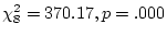
It is interesting to compare the results of the ACE model in
Table 6.11 with those of the ACES model in
Table 6.12. We see that the estimates of and are
identical in the two tables, accounting for  % and
% and
 % of the total variance, respectively. However, in the
first table the estimate of
% of the total variance, respectively. However, in the
first table the estimate of  , accounting for 47% of the
variance. In the analysis with age however,
, accounting for 47% of the
variance. In the analysis with age however,  and accounts
for 29% of variance, and age accounts for
and accounts
for 29% of variance, and age accounts for  . Thus, we
have partitioned our original estimate of 47% due to shared
environment into 18% due to age regression and the remaining 29% due
to `genuine' cultural differences. If we choose, we may recalculate
the proportions of variance due to
. Thus, we
have partitioned our original estimate of 47% due to shared
environment into 18% due to age regression and the remaining 29% due
to `genuine' cultural differences. If we choose, we may recalculate
the proportions of variance due to  , and , as if we were
estimating them from a sample of uniform age -- assuming of course
that the causes of variation do not vary with age (see
Chapter 9). Thus, genetic variance now accounts for
, and , as if we were
estimating them from a sample of uniform age -- assuming of course
that the causes of variation do not vary with age (see
Chapter 9). Thus, genetic variance now accounts for
 % and shared environment variance is estimated to be
 %.
Our analysis suggests that cultural differences are indeed important
in determining individual differences in social attitudes. However,
before accepting this result too readily, we should reflect that
estimates of shared environment may not only be inflated by age
regression, but also by the effects of assortative mating -- the
tendency of like to marry like. Since there is known to be
considerable assortative mating for conservatism (spouse correlations
are typically greater than 0.6), it is possible that a substantial
part of our estimate of
%.
Our analysis suggests that cultural differences are indeed important
in determining individual differences in social attitudes. However,
before accepting this result too readily, we should reflect that
estimates of shared environment may not only be inflated by age
regression, but also by the effects of assortative mating -- the
tendency of like to marry like. Since there is known to be
considerable assortative mating for conservatism (spouse correlations
are typically greater than 0.6), it is possible that a substantial
part of our estimate of  may arise from this source
(Martin et al.,
1986). This issue will be discussed in greater detail in
Chapter .
Age is a somewhat unusual variable since it is perfectly correlated in
both MZ and DZ twins (so long as we measure the members of a pair at
the same time). There are relatively few variables that can be
handled in the same way, partly because we have assumed a strong model
that age causes variability in the observed phenotype. Thus,
for example, it would be inappropriate to model length of time spent
living together as a cause of cancer, even though cohabitation may
lead to greater similarity between twins. In this case a more
suitable model would be one in which the shared environment components
are more highly correlated the longer the twins have been living
together. Such a model would predict greater twin similarity, but
would not predict correlation between cohabitation and cancer. Some
further discussion of this type of model is given in
Section in the context of data-specific models.
One group of variables that may be treated in a similar way to the
present treatment of age consists of maternal gestation factors.
Vlietinck et al. (1989) fitted a model in
which both gestational age and maternal age predicted birthweight in
twins.
Finally we note that at a technical level, age and similar putative
causal agents might most appropriately be treated as
may arise from this source
(Martin et al.,
1986). This issue will be discussed in greater detail in
Chapter .
Age is a somewhat unusual variable since it is perfectly correlated in
both MZ and DZ twins (so long as we measure the members of a pair at
the same time). There are relatively few variables that can be
handled in the same way, partly because we have assumed a strong model
that age causes variability in the observed phenotype. Thus,
for example, it would be inappropriate to model length of time spent
living together as a cause of cancer, even though cohabitation may
lead to greater similarity between twins. In this case a more
suitable model would be one in which the shared environment components
are more highly correlated the longer the twins have been living
together. Such a model would predict greater twin similarity, but
would not predict correlation between cohabitation and cancer. Some
further discussion of this type of model is given in
Section in the context of data-specific models.
One group of variables that may be treated in a similar way to the
present treatment of age consists of maternal gestation factors.
Vlietinck et al. (1989) fitted a model in
which both gestational age and maternal age predicted birthweight in
twins.
Finally we note that at a technical level, age and similar putative
causal agents might most appropriately be treated as  -variables in
a multiple regression model. Thus the observed covariance of the
-variables is incorporated directly into the expected matrix, so
that the analysis of the remaining
-variables in
a multiple regression model. Thus the observed covariance of the
-variables is incorporated directly into the expected matrix, so
that the analysis of the remaining 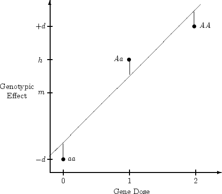 -variables is conditional on the
covariance of the -variables. This type of approach is free of
distributional assumptions for the -variables, and is analogous to
the analysis of covariance. However, when we fit a model that
estimates a single parameter for the variance of age in each group,
the estimated and observed variances are generally equal, so the same
results are obtained.
-variables is conditional on the
covariance of the -variables. This type of approach is free of
distributional assumptions for the -variables, and is analogous to
the analysis of covariance. However, when we fit a model that
estimates a single parameter for the variance of age in each group,
the estimated and observed variances are generally equal, so the same
results are obtained.
Next: 7 Power and Sample
Up: 6 Univariate Analysis
Previous: 1 Major Depressive Disorder
Index
Jeff Lessem
2002-03-21