Next: 1 Application to CBC
Up: 8 Social Interaction
Previous: 2 Basic Univariate Model
Index
3 Sibling Interaction Model
Suppose that we are considering a phenotype like number of cigarettes
smoked. For the sake of exposition we will set aside questions about
the appropriate scale of measurement, what to do about non-smokers and
so on, and assume that there is a well-behaved quantitative variable,
which we can call `smoking' for short. What we want to specify is the
influence of one sibling's (twin's) smoking on the other sibling's
(cotwin's) smoking. Figure 8.2 shows a path diagram which
extends the basic univariate model for twins to
Figure 8.2:
Path diagram for univariate twin data, incorporating sibling
interaction.
 |
include a path of magnitude  from each twin's smoking to the
cotwin. If the path is positive then the sibling interaction is
essentially cooperative, i.e., the more
(less) one twin smokes the more (less) the cotwin will smoke as a
consequence of this direct influence. We can easily conceive of a
highly plausible mechanism for this kind of influence when twins are
cohabiting; as a twin lights up she offers her cotwin a cigarette. If
the path is negative then the sibling interaction is essentially
competitive. The more (less) one twin smokes the less (more) the
cotwin smokes. Although such competition contributes negatively to
the covariance between twins, it may well not override the positive
covariance resulting from shared familial factors. Thus, even in the
presence of competition the observed phenotypic covariation may still
be positive. If interactions are cooperative in some situations and
competitive in others, our analyses will reveal the predominant mode.
But before considering the detail of our expectations, let us look
more closely at how the model is specified. The linear model is now:
from each twin's smoking to the
cotwin. If the path is positive then the sibling interaction is
essentially cooperative, i.e., the more
(less) one twin smokes the more (less) the cotwin will smoke as a
consequence of this direct influence. We can easily conceive of a
highly plausible mechanism for this kind of influence when twins are
cohabiting; as a twin lights up she offers her cotwin a cigarette. If
the path is negative then the sibling interaction is essentially
competitive. The more (less) one twin smokes the less (more) the
cotwin smokes. Although such competition contributes negatively to
the covariance between twins, it may well not override the positive
covariance resulting from shared familial factors. Thus, even in the
presence of competition the observed phenotypic covariation may still
be positive. If interactions are cooperative in some situations and
competitive in others, our analyses will reveal the predominant mode.
But before considering the detail of our expectations, let us look
more closely at how the model is specified. The linear model is now:
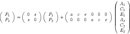
In matrix form we have
or
In this form the B matrix is a square matrix with the number of
rows and columns equal to the number of dependent variables.
The leading diagonal of the B matrix contains
zeros. The element in row  and column
  represents the path from
the
represents the path from
the  dependent variable to the
  dependent variable.
From this equation we can deduce, as shown in more detail below, that:
dependent variable.
From this equation we can deduce, as shown in more detail below, that:
Subsections
Next: 1 Application to CBC
Up: 8 Social Interaction
Previous: 2 Basic Univariate Model
Index
Jeff Lessem
2002-03-21