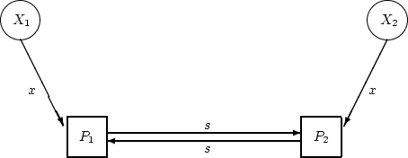
 |
(47) | ||
| (48) |
![[*]](crossref.png) , we can rearrange this
equation, as before:
, we can rearrange this
equation, as before:
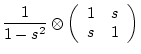
| (49) | |||
| (50) | |||
| (51) |
) we showed how the covariance matrix could be
computed from the raw data matrix 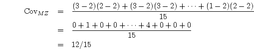 so the matrix is:
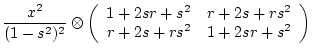 and
and | Source | Variance | Covariance |
| Additive genetic |
|
|
| Dominance genetic |
|
|
| Shared environment |
|
|
| Non-shared environment |
|
|