

Next: 2 Common Pathway Model
Up: 5 Common vs. Independent
Previous: 5 Common vs. Independent
Index
Inspection of the correlation matrices in Table 10.10 reveals
that the presence of any one of the symptoms is associated with an
increased risk of the others within an individual (hence the concept
of ``atopy''). All four symptoms show higher MZ correlations
( ,
,  ,
,  ,
,  ) than DZ correlations in liability
(
 ,
,  ,
,  ,
,  ) and there is a hint of genetic
dominance (or epistasis) for asthma and dust allergy (DZ correlations
less than half their MZ counterparts). Preliminary multivariate
analysis suggests that dominance is acting at the level of a common
factor influencing all symptoms, rather than as specific dominance
of these symptoms is shown in the path diagram of
Figure 10.3
Figure 10.3:
Independent pathway
model for four variables. All labels for path-coefficients have been
omitted. All four correlations at the bottom of the figure are fixed at 1
for MZ and .5 for DZ twins.
 |
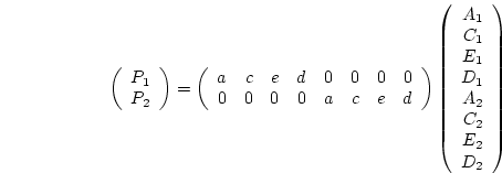
Because each of the three common factors ( ) has its own paths
to each of the four variables, this has been called the
independent pathway model (Kendler
et al., 1987) or the biometric factors model
(McArdle and Goldsmith, 1990).
This is translated into Mx in the
Appendix
 ![[*]](crossref.png) script. The specification of this example is
very similar to the multivariate genetic factor model described earlier in
this chapter. The three common factors are specified in
script. The specification of this example is
very similar to the multivariate genetic factor model described earlier in
this chapter. The three common factors are specified in
nvar 1 matrices
 X, W and Z, where nvar
is defined as 4, representing the four atopy measures. The genetic and
environmental specifics are estimated in nvar
nvar
matrices G and F. The genetic, dominance and specific
environmental covariance matrices are then calculated in the algebra
section. The rest of the script is virtually identical to that for the
univariate model.
One important new feature of the model shown in Figure 10.3
is the treatment of variance specific to each variable. Such residual
variance does not generally receive much attention in regular non-genetic
factor analysis, for at least two reasons. First, the primary goal of
factor analysis (and of many multivariate methods) is to understand the
covariance between variables in terms of reduced number of factors. Thus
the residual, variable specific, components are not the focus. A second
reason is that with phenotypic factor analysis, there is simply no
information very similar to further decompose the variable specific
variance. However, in the case of data on groups of relatives, we have
two parallel goals of understanding not only the within-person covariance
for different variables, but also the across-relatives covariance
structure both within and across variables. The genetic and environmental
factor structure at the top of Figure 10.2 addresses the
genetic and environmental components of variance common to the different
variables. However, there remains information to discriminate between
genetic and environmental components of the residuals, which in essence
answers the question of whether family members correlate for the variable
specific portions of variance.
A second important difference in this example -- using correlation
matrices in which diagonal variance elements are standardized to one --
is that the degrees of freedom available for
model testing are different from the case of fitting to covariance
matrices in which all  elements are available, where
  is the
number of input variables. We encountered this difference in the
univariate case in Section 6.3.1, but it is slightly more
complex in multivariate analysis. For correlation matrices, since the
  diagonal elements are fixed to one, we apparently have
  fewer
degrees of freedom than if we were fitting to covariances, where
  is
the number of data groups. However, since for a given variable the sum of
squared estimates always equals unity (within rounding error), it is
apparent that not all the parameters are free, and we may conceptualize
the unique environment specific standard deviations (i.e., the
  's) as
being obtained as the square roots of one minus the sum of squares of all
the other estimates. Since there are
  (number of variables) such
constrained estimates, we actually have
  more degrees of freedom than
the above discussion indicates, the correct adjustment to the degrees of
freedom when fitting multivariate genetic models to correlation matrices
is
 . Since in most applications
  , the adjustment
is usually
  . In our example
  and the adjustment is indicated by
the option
 DFreedom=-12. (Note that the DFreedom adjustment
applies for the goodness-of-fit chi-squared for the whole problem, not
just the adjustment for that group).
Edited highlights of the Mx output are shown below and the goodness-of-fit
chi-squared indicates an acceptable fit to the data. The adjustment of
 to the degrees of freedom which would be available were we working
with covariance matrices (72) leaves 60 statistics. We have to estimate
 factor loadings and
  specific loadings (20
parameters in all), so there are
  d.f. It is a wise precaution
always to go through this calculation of degrees of freedom -- not
because Mx is likely to get them wrong, but as a further check that the
model has been specified correctly.
Table 10.11:
Parameter estimates from the independent pathway model for atopy
| |
|
|
|
|
|
| |
 |
 |
 |
 |
 |
| Asthma |
.320 |
.431 |
.466 |
.441 |
.548 |
| Hayfever |
.494 |
.772 |
.095 |
.000 |
.388 |
| Dust Allergy |
.660 |
.516 |
.431 |
.297 |
-.159 |
| Eczema |
.092 |
.221 |
.260 |
.712 |
.606 |
 , 40 df, p=.540 , 40 df, p=.540 |
We can test variations of the above model by dropping the common
factors one at a time, or by setting additive genetic specifics to
zero. This is easily done by dropping the appropriate elements. Note
that fixing  specifics to zero usually results in model failure
since it generates singular expected covariance matrices
(
 )
)![[*]](footnote.png) . Neither does it make biological sense
since it is tantamount to saying that a variable can be measured
without error; it is hard to think of a single example of this in
nature! We could also elaborate the model by specifying a third
source of specific variance components, or by substituting shared
environment for dominance, either as a general factor or as specific
variance components.
. Neither does it make biological sense
since it is tantamount to saying that a variable can be measured
without error; it is hard to think of a single example of this in
nature! We could also elaborate the model by specifying a third
source of specific variance components, or by substituting shared
environment for dominance, either as a general factor or as specific
variance components.


Next: 2 Common Pathway Model
Up: 5 Common vs. Independent
Previous: 5 Common vs. Independent
Index
Jeff Lessem
2002-03-21
![[*]](crossref.png) script. The specification of this example is
very similar to the multivariate genetic factor model described earlier in
this chapter. The three common factors are specified in
script. The specification of this example is
very similar to the multivariate genetic factor model described earlier in
this chapter. The three common factors are specified in
 )
)![[*]](footnote.png) . Neither does it make biological sense
since it is tantamount to saying that a variable can be measured
without error; it is hard to think of a single example of this in
nature! We could also elaborate the model by specifying a third
source of specific variance components, or by substituting shared
environment for dominance, either as a general factor or as specific
variance components.
. Neither does it make biological sense
since it is tantamount to saying that a variable can be measured
without error; it is hard to think of a single example of this in
nature! We could also elaborate the model by specifying a third
source of specific variance components, or by substituting shared
environment for dominance, either as a general factor or as specific
variance components.