


Next: 4 Terminology for Types
Up: 3 Ordinal Data Analysis
Previous: 2 Bivariate Normal Distribution
Index
3 Testing the Normal Distribution Assumption
The problem of having no degrees of freedom to test the goodness of fit of
the bivariate normal distribution to two binary variables is solved when
we have at least three categories in one variable and at least two in
the other. To illustrate this point, compare the contour plots shown
in Figure 2.4 in which two thresholds have been specified for
Figure 2.4:
Contour plots of a
bivariate normal distribution with correlation .9 (top) and a
mixture of bivariate normal distributions, one with
.9 correlation and the other with -.9 correlation (bottom). Two thresholds in each
dimension are shown.
 |
the two variables. With the bivariate normal distribution, there is
a very strong pattern imposed on the relative magnitudes of the cells
on the diagonal and elsewhere. There is a similar set of constraints
with the mixture of normals, but quite different predictions are made
about the off-diagonal cells; all four corner cells would have an appreciable
frequency given a sufficient sample size, and probably in excess of that in
each of the four
cells in the middle of each side [e.g., (1,2)]. The bivariate normal distribution could
never be adjusted to perfectly predict the cell proportions obtained from
the mixture of distributions.
This intuitive idea of opportunities for
failure translates directly into the concept of degrees of freedom. When we
use a bivariate normal liability model to predict the proportions in a
contingency table with  rows and
  columns, we use
  thresholds for
the rows,
thresholds for
the rows,  thresholds for the columns, and one parameter for the
correlation in liability, giving
thresholds for the columns, and one parameter for the
correlation in liability, giving  in total. The table itself contains
 proportions, neglecting the total sample size as above. Therefore we
have degrees of freedom equal to:
proportions, neglecting the total sample size as above. Therefore we
have degrees of freedom equal to:
 |
|
|
(5) |
The discrepancy between the frequencies predicted by the model and those
actually observed in the data can be measured using the 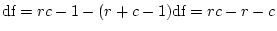 statistic
given by:
statistic
given by:
Given a large enough sample, the model's failure to
predict the observed data would be reflected in a
significant for the goodness of fit.
In principle, models could be fitted by maximum likelihood directly to
contingency tables, employing the observed and expected cell proportions. This
approach is general and flexible, especially for the multigroup case --
the programs LISCOMP (Muthén, 1987) and Mx (Neale, 1991) use the method --
but it is currently limited by computational
considerations. When we move from two variables to larger examples involving
many variables, integration of the multivariate normal distribution (which has
to be done numerically) becomes extremely time-consuming, perhaps increasing by
a factor of ten or so for each additional variable.
An alternative approach to this
problem is to use PRELIS 2 to compute each
correlation in a pairwise fashion, and to compute a weight matrix. The weight
matrix is an estimate of the variances and covariances of the correlations.
The variances of the correlations certainly have some intuitive appeal, being a
measure of how precisely each correlation is estimated. However, the idea of a
correlation correlating with another correlation may seem strange to a newcomer
to the field. Yet this covariation between correlations is precisely what we
need in order to represent how much additional information the second
correlation supplies over and above that provided by the first correlation.
Armed with these two types of summary statistics -- the correlation matrix and
the covariances of the correlations, we may fit models using a structural
equation modeling package such as Mx or LISREL, and make statistical inferences from
the goodness of fit of the model.
It is also possible to use the bivariate normal liability distribution to
infer the patterns of statistics that would be observed if ordinal and
continuous variables were correlated.
Essentially, there are specific predictions made about the expected
mean and variance of the continuous variable in each of the categories of the
ordinal variable. For example, the continuous variable means are predicted to increase
monotonically across the categories if there is a correlation between the
liabilities. An observed pattern of a high mean in category 1, low in category
2 and high again in category 3 would not be consistent with the model.
The number of parameters used to describe this model for an ordinal variable
with categories is 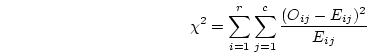 , since we use for the thresholds, one each
for the mean and variance of the continuous variable, and one for the
covariance between the two variables. The observed statistics involved are the
proportions in the cells (less one because the final proportion may be obtained
by subtraction from 1) and the mean and variance of the continuous variable in
each category. Therefore we have:
, since we use for the thresholds, one each
for the mean and variance of the continuous variable, and one for the
covariance between the two variables. The observed statistics involved are the
proportions in the cells (less one because the final proportion may be obtained
by subtraction from 1) and the mean and variance of the continuous variable in
each category. Therefore we have:
So the number of degrees of freedom for such a test is  where is the
number of categories.
where is the
number of categories.
Next: 4 Terminology for Types
Up: 3 Ordinal Data Analysis
Previous: 2 Bivariate Normal Distribution
Index
Jeff Lessem
2002-03-21