


Next: 2 Breeding Experiments: Gametic
Up: 3 Biometrical Genetics
Previous: 3 Biometrical Genetics
Index
The principles of biometrical and quantitative genetics lie at the
heart of virtually all of the statistical models examined in this
book. Thus, an understanding of biometrical genetics is fundamental
to our statistical approach to twin and family data. Biometrical
models relate the ``latent,'' or unobserved, variables of our
structural models to the functional effects of genes. It is these
effects, based on the principles of Mendelian genetics, that give our structural models a degree of validity quite unusual in the social sciences.
The purpose of this chapter is to provide a brief introduction to
biometrical models. Extensive treatments of the subject have been
provided by Mather and Jinks (1982) and Falconer (1990). Here we employ
the notation of Mather and Jinks.
Before we begin our discussion of biometrical genetics, we must
describe some of the terms that are encountered frequently in
biometrical and classical genetic discourse. For the present
purposes, we use the term gene in reference to a
``unit factor of inheritance'' that influences an observable trait or
traits, following the earlier usage by Fuller and Thompson (1978).
Observable characteristics are referred to as
phenotypes. The site of a gene on a chromosome is
known as the locus. Alleles
are alternative forms of a gene that occupy the same locus on a
chromosome. They often are symbolized as A and a or
B and b or  and
and  . The simplest system for a
segregating locus involves only two alleles (A and a), but
there also may be a large number of alleles in a system. For example,
the HLA locus on chromosome 6 is known to have 18 alleles at the A
locus, 41 alleles at the B locus, 8 at C, about 20 at DR, 3 at DQ, and
6 at DP (Bodmer 1987). Nevertheless, if one or two alleles are much
more frequent than the others, a two-allele system provides a useful
approximation and leads to an accurate account for the phenotypic
variation and covariation with which we are concerned. The
genotype is the chromosomal complement of alleles
for an individual. At a single locus (with two alleles) the genotype
may be symbolized AA, Aa, or aa; if we consider multiple
loci the genotype of an individual may be written as AABB, AABb,
AAbb, AaBB, AaBb, Aabb, aaBB, aaBb, or aabb, in the case of
two loci, for example. Homozygosity refers to
a state of identical alleles at corresponding loci on homologous
chromosomes; for example, AA or aa for one locus, or
AABB, aabb, AAbb, or aaBB for two loci. In
contrast, heterozygosity refers to a state
of unlike alleles at corresponding loci, Aa or AaBb, for
example. When numeric or symbolic values are assigned to specific
genotypes they are called genotypic
values. The additive
value of a gene is the sum of the
average effects of the individual alleles. Dominance
deviations refer to the extent to which
genotypes differ from the additive genetic value. A system in which
multiple loci are involved in the expression of a single trait is
called polygenic (``many genes''). A
pleiotropic system (``many growths'') is one
in which the same gene or genes influence more than one trait.
Biometrical models are based on the measurable effects of different
genotypes that arise at a segregating locus, which are summed across
all of the loci that contribute to a continuously varying trait. The
number of loci generally is not known, but it is usual to assume that
a relatively large number of genes of equivalent effect are at work.
In this way, the categories of Mendelian genetics that lead to
binomial distributions for traits in the population tend toward
continuous distributions such as the normal curve. Thus, the
statistical parameters that describe this model are those of
continuous distributions, including the first moment, or the mean;
second moments, or variances, covariances, and correlation
coefficients; and higher moments such as measures of skewness where
these are appropriate. This polygenic model was originally developed
by Sir Ronald Fisher in his classic paper
``The correlation between relatives on the supposition of
Mendelian inheritance'' (Fisher, 1918), in
which he reconciled Galtonian biometrics with Mendelian genetics. One
interesting feature of the polygenic biometrical model is that it
predicts normal distributions for traits when very many loci are
involved and their effects are combined with a multitude of
environmental influences. Since the vast majority of biological and
behavioral traits approximate the normal distribution, it is an
inherently plausible model for the geneticist to adopt. We might
note, however, that although the normality expected for a polygenic
system is statistically convenient as well as empirically appropriate,
none of the biometrical expectations with which we shall be concerned
depend on how many or how few genes are involved. The expectations
are equally valid if there are are only one or two genes, or indeed no
genes at all.
In the simplest two-allele system (A and a) there
are two parameters that define the measurable effects of the three
possible genotypes, AA, Aa, and aa. These parameters are
. The simplest system for a
segregating locus involves only two alleles (A and a), but
there also may be a large number of alleles in a system. For example,
the HLA locus on chromosome 6 is known to have 18 alleles at the A
locus, 41 alleles at the B locus, 8 at C, about 20 at DR, 3 at DQ, and
6 at DP (Bodmer 1987). Nevertheless, if one or two alleles are much
more frequent than the others, a two-allele system provides a useful
approximation and leads to an accurate account for the phenotypic
variation and covariation with which we are concerned. The
genotype is the chromosomal complement of alleles
for an individual. At a single locus (with two alleles) the genotype
may be symbolized AA, Aa, or aa; if we consider multiple
loci the genotype of an individual may be written as AABB, AABb,
AAbb, AaBB, AaBb, Aabb, aaBB, aaBb, or aabb, in the case of
two loci, for example. Homozygosity refers to
a state of identical alleles at corresponding loci on homologous
chromosomes; for example, AA or aa for one locus, or
AABB, aabb, AAbb, or aaBB for two loci. In
contrast, heterozygosity refers to a state
of unlike alleles at corresponding loci, Aa or AaBb, for
example. When numeric or symbolic values are assigned to specific
genotypes they are called genotypic
values. The additive
value of a gene is the sum of the
average effects of the individual alleles. Dominance
deviations refer to the extent to which
genotypes differ from the additive genetic value. A system in which
multiple loci are involved in the expression of a single trait is
called polygenic (``many genes''). A
pleiotropic system (``many growths'') is one
in which the same gene or genes influence more than one trait.
Biometrical models are based on the measurable effects of different
genotypes that arise at a segregating locus, which are summed across
all of the loci that contribute to a continuously varying trait. The
number of loci generally is not known, but it is usual to assume that
a relatively large number of genes of equivalent effect are at work.
In this way, the categories of Mendelian genetics that lead to
binomial distributions for traits in the population tend toward
continuous distributions such as the normal curve. Thus, the
statistical parameters that describe this model are those of
continuous distributions, including the first moment, or the mean;
second moments, or variances, covariances, and correlation
coefficients; and higher moments such as measures of skewness where
these are appropriate. This polygenic model was originally developed
by Sir Ronald Fisher in his classic paper
``The correlation between relatives on the supposition of
Mendelian inheritance'' (Fisher, 1918), in
which he reconciled Galtonian biometrics with Mendelian genetics. One
interesting feature of the polygenic biometrical model is that it
predicts normal distributions for traits when very many loci are
involved and their effects are combined with a multitude of
environmental influences. Since the vast majority of biological and
behavioral traits approximate the normal distribution, it is an
inherently plausible model for the geneticist to adopt. We might
note, however, that although the normality expected for a polygenic
system is statistically convenient as well as empirically appropriate,
none of the biometrical expectations with which we shall be concerned
depend on how many or how few genes are involved. The expectations
are equally valid if there are are only one or two genes, or indeed no
genes at all.
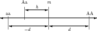
In the simplest two-allele system (A and a) there
are two parameters that define the measurable effects of the three
possible genotypes, AA, Aa, and aa. These parameters are
 , which is twice the measured difference between the homozygotes
AA and aa, and
, which is twice the measured difference between the homozygotes
AA and aa, and  , which defines the measured effect of
the heterozygote Aa, insofar as it does not fall exactly between
the homozygotes. The point between the two homozygotes is
, which defines the measured effect of
the heterozygote Aa, insofar as it does not fall exactly between
the homozygotes. The point between the two homozygotes is  , the
mean effect of homozygous genotypes. We refer to the parameters
and as genotypic effects. The
scaling of the three genotypes is shown in Figure 3.1.
, the
mean effect of homozygous genotypes. We refer to the parameters
and as genotypic effects. The
scaling of the three genotypes is shown in Figure 3.1.
Figure 3.1:
The and increments of the gene difference  -
-  .
.
 may lie on either side of and the sign of will vary
accordingly; in the case illustrated would be negative. (Adapted from Mather and Jinks, 1977, p. 32).
may lie on either side of and the sign of will vary
accordingly; in the case illustrated would be negative. (Adapted from Mather and Jinks, 1977, p. 32).
 |
To make the simple two-allele model concrete, let us imagine that we
are talking about genes that influence adult stature. Let us assume
that the normal range of height for males is from 4 feet 10 inches to
6 feet 8 inches; that is, about 22 inches![[*]](footnote.png) . And let us assume that each somatic
chromosome has one gene of roughly equivalent effect. Then, roughly
speaking, we are thinking in terms of loci for which the homozygotes
contribute
. And let us assume that each somatic
chromosome has one gene of roughly equivalent effect. Then, roughly
speaking, we are thinking in terms of loci for which the homozygotes
contribute
 inch (from the midpoint), depending on
whether they are AA, the increasing homozygote, or aa, the
decreasing homozygotes. In reality, although some loci may contribute
greater effects than this, others will almost certainly contribute
less; thus we are talking about the kind of model in which any
particular polygene is having an effect that would be difficult to
detect by the methods of classical genetics. Similarly, while the
methods of linkage analysis may be appropriate for a number of
quantitative loci, it seems unlikely that the majority of causes of
genetic variation would be detectable by these means. The biometrical
approach, being founded upon an assumption that inheritance may be
polygenic, is designed to elucidate sources of genetic variation is
these types of systems.
inch (from the midpoint), depending on
whether they are AA, the increasing homozygote, or aa, the
decreasing homozygotes. In reality, although some loci may contribute
greater effects than this, others will almost certainly contribute
less; thus we are talking about the kind of model in which any
particular polygene is having an effect that would be difficult to
detect by the methods of classical genetics. Similarly, while the
methods of linkage analysis may be appropriate for a number of
quantitative loci, it seems unlikely that the majority of causes of
genetic variation would be detectable by these means. The biometrical
approach, being founded upon an assumption that inheritance may be
polygenic, is designed to elucidate sources of genetic variation is
these types of systems.
Next: 2 Breeding Experiments: Gametic
Up: 3 Biometrical Genetics
Previous: 3 Biometrical Genetics
Index
Jeff Lessem
2002-03-21