Next: 3 Derivation of Expected
Up: 3 Biometrical Genetics
Previous: 1 Introduction and Description
Index
2 Breeding Experiments: Gametic Crosses
The methods of biometrical genetics are best understood through
controlled breeding experiments with
inbred strains, in which the results are simple and intuitively
obvious. Of course, in the present context we are dealing with
continuous variation in humans, where inbred strains do not exist and
controlled breeding experiments are impossible. However, the simple
results from inbred strains of animals apply directly, albeit in more
complex form, to those of free mating organisms such as humans. We
feel an appreciation of the simple results from controlled breeding
experiments provides insight and lends credibility to the application
of the models to human beings.
Let us consider a cross between two inbred parental strains,  and
and
 , with genotypes AA and aa, respectively. Since
individuals in the strain can produce gametes with only the
A allele, and individuals can produce only a gametes,
all of the offspring of such a mating will be heterozygotes, Aa,
forming what Gregor Mendel referred to as the
``first filial,'' or
, with genotypes AA and aa, respectively. Since
individuals in the strain can produce gametes with only the
A allele, and individuals can produce only a gametes,
all of the offspring of such a mating will be heterozygotes, Aa,
forming what Gregor Mendel referred to as the
``first filial,'' or  generation. A cross between two
individuals generates what he referred to as the ``second filial''
generation, or
generation. A cross between two
individuals generates what he referred to as the ``second filial''
generation, or  , and it may be shown that this generation
comprises
, and it may be shown that this generation
comprises  individuals of genotype AA,
aa, and
individuals of genotype AA,
aa, and  Aa. Mendel's first
law, the law of segregation, states
that parents with genotype Aa will produce the
gametes A and a in equal proportions. The
pioneer Mendelian geneticist Reginald Punnett
developed a device known as the Punnett square, which he found
useful in teaching Mendelian genetics to Cambridge undergraduates,
that gives the proportions of genotypes that
will arise when these gametes unite at random.
(Random unions of gametes occur under the condition of random mating
among individuals). The result of other matings such as
Aa. Mendel's first
law, the law of segregation, states
that parents with genotype Aa will produce the
gametes A and a in equal proportions. The
pioneer Mendelian geneticist Reginald Punnett
developed a device known as the Punnett square, which he found
useful in teaching Mendelian genetics to Cambridge undergraduates,
that gives the proportions of genotypes that
will arise when these gametes unite at random.
(Random unions of gametes occur under the condition of random mating
among individuals). The result of other matings such as
 , the first backcross,
  , and more complex
combinations may be elucidated in a similar manner. A simple usage of
the Punnett square is shown in Table 3.1 for the mating of
two heterozygous parents in a two-allele system. The gamete
frequencies in Table 3.1 (shown outside the box) are known as
gene or allelic frequencies, and they
give rise to the genotypic frequencies
by a simple product of independent
probabilities. It is this assumption of independence based on random
mating that makes the biometrical model straightforward and tractable
in more complex situations, such as random mating in populations where
the gene frequencies are unequal. It also forms a simple basis for
considering the more complex effects of non-random mating, or
assortative mating, which are known to be important in human
populations.
, and more complex
combinations may be elucidated in a similar manner. A simple usage of
the Punnett square is shown in Table 3.1 for the mating of
two heterozygous parents in a two-allele system. The gamete
frequencies in Table 3.1 (shown outside the box) are known as
gene or allelic frequencies, and they
give rise to the genotypic frequencies
by a simple product of independent
probabilities. It is this assumption of independence based on random
mating that makes the biometrical model straightforward and tractable
in more complex situations, such as random mating in populations where
the gene frequencies are unequal. It also forms a simple basis for
considering the more complex effects of non-random mating, or
assortative mating, which are known to be important in human
populations.
Table 3.1:
Punnett square for mating
between two heterozygous parents.
| |
|
Male Gametes |
| |
|
 |
 |
| Female Gametes |
|
 |
 |
| |
|
|
 |
In the simple case of equal gene frequencies as we have in an
population, it is easily shown that random mating over successive
generations changes neither the gene nor genotype frequencies of the
population. Male and female gametes of the type A and a
from an population are produced in equal proportions so that
random mating may be represented by the same Punnett square as given
in Table 3.1, which simply reproduces a population with
identical structure to the from which we started. This
remarkable result is known as Hardy-Weinberg equilibrium and is
the cornerstone of quantitative and population genetics. From this
result, the effects of non-random mating and other forces that change
populations, such as natural selection, migration, and mutation, may
be deduced. Hardy-Weinberg equilibrium is achieved in one
generation and applies whether or not the gene frequencies are equal
and whether or not there are more than two alleles. It also holds
among polygenic loci, linked or unlinked, although in these cases
joint equilibrium depends on a number of generations of random mating.
For our purposes the genotypic frequencies from the Punnett square are
important because they allow us to calculate the simple first and
second moments of the phenotypic distribution that result from genetic
effects; namely, the mean and variance of the phenotypic trait. The
genotypes, frequencies, and genotypic effects of the biometrical model
in Table 3.1 are shown below, and from these we can calculate
the mean and variance.
Genotype ( ) ) |
 |
 |
 |
Frequency ( ) ) |
|
|
|
Genotypic effect ( ) ) |
 |
 |
 |
The mean effect of the A locus is obtained by summing the
products of the frequencies and genotypic effects in the following
manner:
The variance of the genetic effects is given by the sum of the
products of the genotypic frequencies and their squared deviations
from the mean![[*]](footnote.png) :
:
For this single locus with equal gene frequencies,
 is
known as the additive genetic variance,
or
is
known as the additive genetic variance,
or  , and
, and
 is known as the dominance variance,
  .
When more than one locus
is involved, perhaps many loci as we envisage in the polygenic model,
Mendel's law of independent
assortment permits the
simple summation of the individual effects of
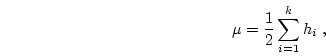
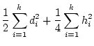
separate loci in both the mean and the variance. Thus, for (
.
When more than one locus
is involved, perhaps many loci as we envisage in the polygenic model,
Mendel's law of independent
assortment permits the
simple summation of the individual effects of
separate loci in both the mean and the variance. Thus, for ( )
multiple loci,
)
multiple loci,
 |
(9) |
and
It is the parameters and that we estimate using the
structural equations in this book.
In order to see how this biometrical model and the equations
estimate and , we need to consider the joint effect of
genes in related individuals. That is, we need to derive expectations
for MZ and DZ covariances in terms of the genotypic frequencies and the
effects of and .
Next: 3 Derivation of Expected
Up: 3 Biometrical Genetics
Previous: 1 Introduction and Description
Index
Jeff Lessem
2002-03-21