


Next: 4 Matrix Algebra
Up: 3 Biometrical Genetics
Previous: 2 Unequal Gene Frequencies
Index
Table 3.3 replicates Table 3.2 employing genotypic
frequencies appropriate to random mating and unequal gene frequencies.
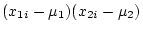
Using the table to calculate covariances among sibling pairs of the three
types, MZ twins, DZ twins, and unrelated siblings, gives
Table 3.3:
Genetic covariance components for MZ, DZ,
and Unrelated Siblings with unequal gene frequencies at a single
locus.
| Genotype |
Effect |
|
Frequency |
| Pair |
 |
 |
|
MZ |
DZ |
U |
 |
 |
|
|
 |
 |
 |
 |
|
 |
|
- |
 |
 |
 |
|
 |
|
-- |
 |
 |
 |
|
|
|
-- |
|
|
 |
|
|
|
 |
 |
 |
 |
|
|
|
-- |
 |
 |
 |
|
|
|
-- |
|
|
 |
|
|
|
-- |
|
|
 |
|
|
|
|
 |
 |
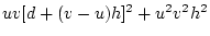
By similar calculations, the expectations for half-siblings and for
parents and their offspring may be shown to be
 and
and
 ,
respectively. That is, these relationships do not reflect dominance
effects. The MZ and DZ resemblances are the primary focus of
this text, but all five relationships we have just discussed may be
analyzed in the extended Mx approaches we discuss in
Chapter
,
respectively. That is, these relationships do not reflect dominance
effects. The MZ and DZ resemblances are the primary focus of
this text, but all five relationships we have just discussed may be
analyzed in the extended Mx approaches we discuss in
Chapter ![[*]](crossref.png) .
With more extensive genetical data, we can assess the effects of
epistasis, or non-allelic interaction, since
the biometrical model may
be extended easily to include such genetic effects. Another
important problem we have not considered is that of assortative
mating, which one might have thought would
introduce insuperable
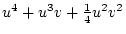
problems for the model. However, once we are working with genotypic
values such as
.
With more extensive genetical data, we can assess the effects of
epistasis, or non-allelic interaction, since
the biometrical model may
be extended easily to include such genetic effects. Another
important problem we have not considered is that of assortative
mating, which one might have thought would
introduce insuperable
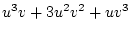
problems for the model. However, once we are working with genotypic
values such as  and
and  , the effects of assortment can be readily
accommodated in the model by means of reverse path analysis (Wright,
1968) and the Pearson-Aitken treatment of selected variables
(Aitken, 1934). Fulker (1988) describes this approach in the context
of Fisher's (1918) model of assortment.
In this chapter, we have given a brief introduction to the biometrical
model that underlies the model fitting approach employed in this book, and
we have indicated how additional genetic complexities may be
accommodated in the model. However, in addition to genetic influences,
we must consider the effects of the environment on any phenotype.
These may be easily accommodated by defining environmental influences
that are common to sib pairs and those that are unique to the
individual. If these environmental effects
are unrelated to the genotype, then the variances due to these
influences simply add to the genetic variances we have just described.
If they are not independent of genotype, as in the case of sibling
interactions and cultural transmission, both of which are likely to
occur in some behavioral phenotypes, then the Mx model may be
suitably modified to account for these complexities, as we describe in
Chapters 8 and .
, the effects of assortment can be readily
accommodated in the model by means of reverse path analysis (Wright,
1968) and the Pearson-Aitken treatment of selected variables
(Aitken, 1934). Fulker (1988) describes this approach in the context
of Fisher's (1918) model of assortment.
In this chapter, we have given a brief introduction to the biometrical
model that underlies the model fitting approach employed in this book, and
we have indicated how additional genetic complexities may be
accommodated in the model. However, in addition to genetic influences,
we must consider the effects of the environment on any phenotype.
These may be easily accommodated by defining environmental influences
that are common to sib pairs and those that are unique to the
individual. If these environmental effects
are unrelated to the genotype, then the variances due to these
influences simply add to the genetic variances we have just described.
If they are not independent of genotype, as in the case of sibling
interactions and cultural transmission, both of which are likely to
occur in some behavioral phenotypes, then the Mx model may be
suitably modified to account for these complexities, as we describe in
Chapters 8 and .
Next: 4 Matrix Algebra
Up: 3 Biometrical Genetics
Previous: 2 Unequal Gene Frequencies
Index
Jeff Lessem
2002-03-21