Next: 4 Summary
Up: 3 Derivation of Expected
Previous: 1 Equal Gene Frequencies
Index
2 Unequal Gene Frequencies
The simple
results for equal gene frequencies described in the previous section
were appreciated by a number of biometricians shortly after the
rediscovery of Mendel's work (Castle, 1903; Pearson, 1904; Yule,
1902). However, it was not until Fisher's
remarkable 1918 paper that the full generality of the biometrical
model was elucidated. Gene frequencies do not have to be equal, nor
do they have to be the same for the various polygenic loci involved in
the phenotype for the simple fractions,  ,
,
 , and
, and  to hold, providing we define
  and
and  appropriately. The algebra is considerably more complicated with
unequal gene frequencies and it is necessary to define carefully what
we mean by and . However, the end result is extremely
simple, which is perhaps somewhat surprising. We give the flavor of
the approach in this section, and refer the interested reader to the
classic texts in this field for further information (Crow and Kimura,
1970; Falconer, 1990; Kempthorne, 1960;
Mather and Jinks, 1982).
We note that the elaboration of this biometrical model and its power
and elegance has been largely responsible for the tremendous strides
in inexpensive plant and animal food production throughout the world,
placing these activities on a firm scientific basis.
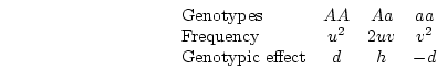
Consider the three genotypes, AA, Aa, and aa, with
genotypic frequencies
appropriately. The algebra is considerably more complicated with
unequal gene frequencies and it is necessary to define carefully what
we mean by and . However, the end result is extremely
simple, which is perhaps somewhat surprising. We give the flavor of
the approach in this section, and refer the interested reader to the
classic texts in this field for further information (Crow and Kimura,
1970; Falconer, 1990; Kempthorne, 1960;
Mather and Jinks, 1982).
We note that the elaboration of this biometrical model and its power
and elegance has been largely responsible for the tremendous strides
in inexpensive plant and animal food production throughout the world,
placing these activities on a firm scientific basis.
Consider the three genotypes, AA, Aa, and aa, with
genotypic frequencies  ,
,  ,
,  :
The proportion of alleles, or gene frequency, is given by
:
The proportion of alleles, or gene frequency, is given by
These expressions derive from the simple fact that the AA genotype
contributes only A alleles and the heterozygote, Aa,
contributes  A and a alleles.
A Punnett square showing the allelic form of gametes
uniting at random gives the genotypic frequencies in terms of the
gene frequencies:
A and a alleles.
A Punnett square showing the allelic form of gametes
uniting at random gives the genotypic frequencies in terms of the
gene frequencies:
| |
Male Gametes |
| |
 A A |
 a a |
| Female Gametes |
A |
 |
 |
| |
a |
|
 |
which yields an alternative representation of the genotypic
frequencies
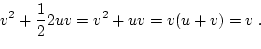
That these genotypic frequencies are in Hardy-Weinberg equilibrium may
be shown by using them to calculate gene frequencies in the new
generation, showing them to be the same, and then reapplying the
Punnett square. Using expression 3.8, substituting
 ,
,  , and
, and  , for , , and , and noting that the
sum of gene frequencies is 1 (
, for , , and , and noting that the
sum of gene frequencies is 1 ( ), we can see that the new gene
frequencies are the same as the old, and that genotypic frequencies
will not change in subsequent generations
), we can see that the new gene
frequencies are the same as the old, and that genotypic frequencies
will not change in subsequent generations
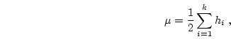
The biometrical model is developed in terms of these equilibrium
frequencies and genotypic effects as
 |
(16) |
The mean and variance of a population with this composition is
obtained in analogous manner to that in 3.1. The mean is
Because the mean is a reasonably complex expression, it is not
convenient to sum weighted deviations to express the variance as in
3.2, instead, we rearrange the variance formula
Applying this formula to the genotypic effects and their frequencies
given in 3.10 above, we obtain
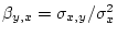
When the variance is arranged in this form, the first term (
![$2uv [d
+ (v-u)h]^2$](img251.png) ) defines the additive genetic
variance, , and the second term
(
) defines the additive genetic
variance, , and the second term
( ) the dominance variance, .
Why this particular arrangement is used to define and
rather than some other may be seen if we introduce the notion of gene dose
and the regression of genotypic effects on this variable, which
essentially is how Fisher proceeded to develop the concepts of
and .
If A is the increasing allele, then we can consider the
three genotypes, AA, Aa, aa, as containing
) the dominance variance, .
Why this particular arrangement is used to define and
rather than some other may be seen if we introduce the notion of gene dose
and the regression of genotypic effects on this variable, which
essentially is how Fisher proceeded to develop the concepts of
and .
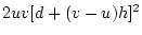
If A is the increasing allele, then we can consider the
three genotypes, AA, Aa, aa, as containing  , , and
doses of the A allele, respectively. The regression of
genotypic effects on these gene doses
is shown in Figure 3.2.
, , and
doses of the A allele, respectively. The regression of
genotypic effects on these gene doses
is shown in Figure 3.2.
Figure 3.2:
Regression of
genotypic effects on gene dosage showing
additive and dominance effects under random mating. The figure is drawn
to scale for
 ,
,  , and
, and
 .
.
 |
The values that enter into the calculation of the slope of
this line are
| Genotype |
AA |
Aa |
aa |
Genotypic effect ( ) ) |
 |
 |
 |
Frequency ( ) ) |
|
|
|
Dose ( ) ) |
2 |
1 |
0 |
From these values the slope of the regression line of
on in Figure 3.2 is given by
 .
In order to calculate
.
In order to calculate
 we need
  , which is
Then,
is
using the variance formula in 3.12.
In order to calculate 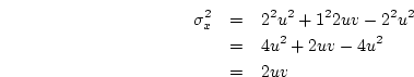 we need to employ the
covariance formula
we need to employ the
covariance formula
 |
(21) |
where  and are defined as in 3.11 and
3.14, respectively. Then,
and are defined as in 3.11 and
3.14, respectively. Then,
Therefore, the slope is
Following standard procedures in regression analysis, we can partition
 into the variance due to the regression and the
variance due to residual.
The former is equivalent to the variance of the expected ;
that is, the variance of the hypothetical points on the line in
Figure 3.2, and the latter is the variance of the difference
between observed and the expected values.
The variance due to regression is
into the variance due to the regression and the
variance due to residual.
The former is equivalent to the variance of the expected ;
that is, the variance of the hypothetical points on the line in
Figure 3.2, and the latter is the variance of the difference
between observed and the expected values.
The variance due to regression is
and we may obtain the residual variance simply by subtracting the
variance due to regression from the total variance of . The
variance of genotypic effects (
) was given in
3.13, and when we subtract
the expression obtained for the variance due to regression
3.18, we obtain the residual variances:
In this representation, genotypic effects are defined in terms of the
regression line and are known as genotypic
values. They are related to
and , the genotypic effects we defined in Figure 3.1, but
now reflect the population mean and gene frequencies of our random
mating population. Defined in this way, the genotypic value ( ) is
) is
 , the additive (
 ) and dominance (
 ) deviations of the
individual.
In the case of
, this table becomes
from which it can be seen that the weighted sum of all 's is zero
(
) deviations of the
individual.
In the case of
, this table becomes
from which it can be seen that the weighted sum of all 's is zero
(
 ).
In this case the additive effect is the same as the genotypic effect
as originally scaled, and the dominance effect is measured around a
mean of
).
In this case the additive effect is the same as the genotypic effect
as originally scaled, and the dominance effect is measured around a
mean of  . This representation
of genotypic value accurately conveys the extreme nature of unusual
genotypes. Let
. This representation
of genotypic value accurately conveys the extreme nature of unusual
genotypes. Let  , an example of complete
dominance. In that case,
, an example of complete
dominance. In that case,
 and
and
 on our scale. Thus, aa genotypes, which form
only
on our scale. Thus, aa genotypes, which form
only  of the population, fall far below the mean of ,
while the remaining
of the population, fall far below the mean of ,
while the remaining  of the population genotypes fall
only slightly above the mean of . Thus, the bulk of the population
appears relatively normal, whereas aa genotypes appear abnormal
or unusual. When dominance is absent (
of the population genotypes fall
only slightly above the mean of . Thus, the bulk of the population
appears relatively normal, whereas aa genotypes appear abnormal
or unusual. When dominance is absent ( ), Aa genotypes,
which form of the population, have a mean of and the
less frequent genotypes AA and aa appear deviant. This
situation is accentuated as the gene frequencies depart from
. For example, with
), Aa genotypes,
which form of the population, have a mean of and the
less frequent genotypes AA and aa appear deviant. This
situation is accentuated as the gene frequencies depart from
. For example, with
 ,
,
 , and
, and  , then AA and Aa combined form
 of the population with a genotypic value of
 , just slightly above
the mean of , whereas the aa genotype has a value of
, just slightly above
the mean of , whereas the aa genotype has a value of
 . In the limiting case of a very rare allele, AA
and Aa tend to , the population mean, while only aa
genotypes take an
extreme value. These values intuitively correspond to our notion of a
rare disorder of extreme effect, such as untreated phenylketonuria (PKU).
The genotypic values and that we employ in the Mx model
have precisely the expectations given above in 3.18 and
3.19, but are summed over all
polygenic loci contributing to the trait. Thus, the biometrical model
gives a precise definition to the latent variables employed in Mx
for the analysis of twin data.
. In the limiting case of a very rare allele, AA
and Aa tend to , the population mean, while only aa
genotypes take an
extreme value. These values intuitively correspond to our notion of a
rare disorder of extreme effect, such as untreated phenylketonuria (PKU).
The genotypic values and that we employ in the Mx model
have precisely the expectations given above in 3.18 and
3.19, but are summed over all
polygenic loci contributing to the trait. Thus, the biometrical model
gives a precise definition to the latent variables employed in Mx
for the analysis of twin data.
Next: 4 Summary
Up: 3 Derivation of Expected
Previous: 1 Equal Gene Frequencies
Index
Jeff Lessem
2002-03-21