Next: 6 Path Models for
Up: 5 Path Analysis and
Previous: 2 Tracing Rules for
Index
5 Path Models for Linear Regression
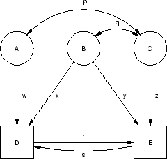
Figure 5.2:
Regression path models with manifest variables.
 |
In this Section we attempt to clarify the conventions, the assumptions
and the tracing rules of path analysis by applying them to regression
models. The path diagram in Figure 5.2a
represents a linear regression model, such as might be used, for
example, to predict systolic blood pressure [SBP],  from sodium
intake
from sodium
intake  . The model asserts that high sodium intake is a
cause, or direct effect,
of high blood pressure (i.e., sodium intake
. The model asserts that high sodium intake is a
cause, or direct effect,
of high blood pressure (i.e., sodium intake  blood
pressure), but that blood pressure also is influenced by other,
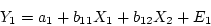
unmeasured (`residual'), factors. The regression equation represented
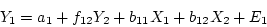
in Figure 5.2a is
blood
pressure), but that blood pressure also is influenced by other,
unmeasured (`residual'), factors. The regression equation represented
in Figure 5.2a is
 |
(26) |
where  is a constant intercept term,
  the regression or
`structural' coefficient, and
the regression or
`structural' coefficient, and  the residual error term or
disturbance term,
which is uncorrelated with . This is indicated by the absence of
a double-headed arrow between and or an indirect common
cause between them [Cov(,) = 0]. The double-headed arrow
from to itself represents the variance of this variable:
Var(
the residual error term or
disturbance term,
which is uncorrelated with . This is indicated by the absence of
a double-headed arrow between and or an indirect common
cause between them [Cov(,) = 0]. The double-headed arrow
from to itself represents the variance of this variable:
Var( ) =
) =  ; the variance of is Var(
 ) =
) =  . In
this example SBP is the dependent variable and sodium intake
is the independent variable.
We can extend the model by adding more independent variables or more
dependent variables or both. The path diagram in Figure 5.2b
represents a multiple regression model, such as might be used if we
were trying to predict SBP () from sodium intake
(), exercise (
. In
this example SBP is the dependent variable and sodium intake
is the independent variable.
We can extend the model by adding more independent variables or more
dependent variables or both. The path diagram in Figure 5.2b
represents a multiple regression model, such as might be used if we
were trying to predict SBP () from sodium intake
(), exercise ( ), and body mass index [BMI] (
 ), allowing
once again for the influence of other residual factors () on
blood pressure. The double-headed arrows between the three
independent variables indicate that correlations are allowed between
sodium intake and exercise (
), allowing
once again for the influence of other residual factors () on
blood pressure. The double-headed arrows between the three
independent variables indicate that correlations are allowed between
sodium intake and exercise ( ), sodium intake and BMI
(
), sodium intake and BMI
( ), and BMI and exercise (
 ). For example, a negative
covariance between exercise and sodium intake might arise if the
health-conscious exercised more and ingested less sodium; positive
covariance between sodium intake and BMI could occur if obese
individuals ate more (and therefore ingested more sodium); and a
negative covariance between BMI and exercise could exist if overweight
people were less inclined to exercise. In this case the regression
equation is
). For example, a negative
covariance between exercise and sodium intake might arise if the
health-conscious exercised more and ingested less sodium; positive
covariance between sodium intake and BMI could occur if obese
individuals ate more (and therefore ingested more sodium); and a
negative covariance between BMI and exercise could exist if overweight
people were less inclined to exercise. In this case the regression
equation is
 |
(27) |
Note that the estimated values for  , and will not
usually be the same as in equation 5.1 due to the inclusion
of additional independent variables in the multiple regression
equation 5.2. Similarly, the only difference between
Figures 5.2a and 5.2b is that we have multiple
independent or predictor variables in Figure 5.2b.
Figure 5.2c represents a multivariate regression model, where
we now have two dependent variables (blood pressure, , and a
measure of coronary artery disease [CAD],
, and will not
usually be the same as in equation 5.1 due to the inclusion
of additional independent variables in the multiple regression
equation 5.2. Similarly, the only difference between
Figures 5.2a and 5.2b is that we have multiple
independent or predictor variables in Figure 5.2b.
Figure 5.2c represents a multivariate regression model, where
we now have two dependent variables (blood pressure, , and a
measure of coronary artery disease [CAD],  ), as well as the same
set of independent variables (case 1). The model postulates that
there are direct influences of sodium intake and exercise on blood
pressure, and of exercise and BMI on CAD, but no direct influence of
sodium intake on CAD, nor of BMI on blood pressure. Because the
variable, exercise, causes both blood pressure, , and coronary
artery disease, , it is termed a common cause of these dependent variables. The
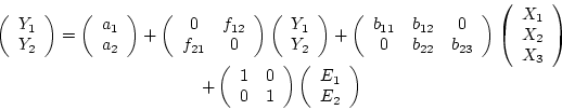
regression equations are
), as well as the same
set of independent variables (case 1). The model postulates that
there are direct influences of sodium intake and exercise on blood
pressure, and of exercise and BMI on CAD, but no direct influence of
sodium intake on CAD, nor of BMI on blood pressure. Because the
variable, exercise, causes both blood pressure, , and coronary
artery disease, , it is termed a common cause of these dependent variables. The
regression equations are
and
 |
(28) |
Here and are the intercept term and error term,
respectively, and and  the regression coefficients for
predicting blood pressure, and
the regression coefficients for
predicting blood pressure, and  ,
,  ,
,  , and
, and  the
corresponding coefficients for predicting coronary artery disease. We
can rewrite equation 5.3 using matrices (see
Chapter 4 on matrix algebra),
the
corresponding coefficients for predicting coronary artery disease. We
can rewrite equation 5.3 using matrices (see
Chapter 4 on matrix algebra),
or, using matrix notation,
where y, a, x, and e are column vectors and
B is a matrix of regression coefficients and I is an
identity matrix.
Note that each variable in the path diagram which has an
arrow pointing to it appears exactly one time on the left side of the
matrix expression.
Figure 5.2d differs from Figure 5.2c only by the
addition of a causal path ( ) from blood pressure to coronary
artery disease, implying the hypothesis that high blood pressure
increases CAD (case 2). The presence of this path also provides a
link between and (
) from blood pressure to coronary
artery disease, implying the hypothesis that high blood pressure
increases CAD (case 2). The presence of this path also provides a
link between and (
 );
this type of process with multiple intervening variables is typically
called an indirect effect (of on ). Thus we see that dependent variables
can be influenced by other dependent variables, as well as by
independent variables. Figure 5.2e adds an additional causal
path from CAD to blood pressure (
);
this type of process with multiple intervening variables is typically
called an indirect effect (of on ). Thus we see that dependent variables
can be influenced by other dependent variables, as well as by
independent variables. Figure 5.2e adds an additional causal
path from CAD to blood pressure (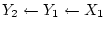 ), thus creating a
`feedback-loop' (hereafter designated as
), thus creating a
`feedback-loop' (hereafter designated as
 ) between CAD and blood pressure. If both
 parameters are positive, the interpretation of the model would
be that high SBP increases CAD and increased CAD in turn increases
SBP. Such reciprocal causation of variables requires special
treatment and is discussed further in Chapters 8
and
parameters are positive, the interpretation of the model would
be that high SBP increases CAD and increased CAD in turn increases
SBP. Such reciprocal causation of variables requires special
treatment and is discussed further in Chapters 8
and ![[*]](crossref.png) . Figure 5.2e implies the structural
equations
. Figure 5.2e implies the structural
equations
and
 |
(29) |
In matrix form, we may write these equations as
i.e.,
Now that some examples of regression models have been described both
in the form of path diagrams and structural equations, we can apply
the tracing rules of path analysis to derive the expected variances
and covariances under the models. The regression models presented in
this chapter are all examples of unstandardized variables. We
illustrate the derivation of the expected variance or covariance
between some variables by applying the tracing rules for
unstandardized variables in Figures 5.2a, 5.2b and
5.2c. As an exercise, the reader may wish to trace some of
the other paths.
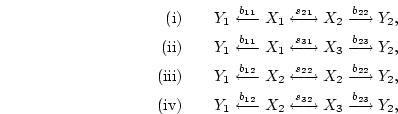
In the case of Figure 5.2a, to derive the expected covariance
between and , we need trace only the path:
yielding an expected covariance of ( ).
Two paths contribute to the expected variance of ,
).
Two paths contribute to the expected variance of ,
yielding an expected variance of of (
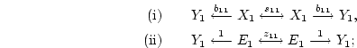 ).
In the case of Figure 5.2b, to derive the expected
covariance of and , we can trace paths:
).
In the case of Figure 5.2b, to derive the expected
covariance of and , we can trace paths:
to obtain an expected covariance of (
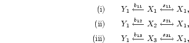 ).
To derive the expected variance of , we can trace paths:
).
To derive the expected variance of , we can trace paths:
yielding a total expected variance of (
 ).
In the case of Figure 5.2c, we may derive the expected
covariance of and as the sum of
).
In the case of Figure 5.2c, we may derive the expected
covariance of and as the sum of
giving [
 ] for the expected covariance. This expectation, and
the preceding ones, can be derived equally (and arguably more easily)
by simple matrix algebra. For example, the expected covariance matrix
(
] for the expected covariance. This expectation, and
the preceding ones, can be derived equally (and arguably more easily)
by simple matrix algebra. For example, the expected covariance matrix
(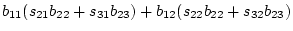 ) for and under the model of
Figure 5.2c is given as
) for and under the model of
Figure 5.2c is given as
in which the elements of B are the paths from the X variables
(columns) to the Y variables (rows); the elements of 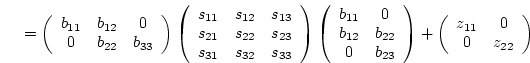 are
the covariances between the independent variables; and the elements of
are
the covariances between the independent variables; and the elements of
 are the residual error variances.
Next: 6 Path Models for
Up: 5 Path Analysis and
Previous: 2 Tracing Rules for
Index
Jeff Lessem
2002-03-21