Next: 8 Summary
Up: 5 Path Analysis and
Previous: 2 Variance Components Model:
Index
7 Identification of Models and Parameters
One key issue with structural equation modeling is whether a model, or
a parameter within a model is
identified. We say that the free
parameters of a model are either (i) overidentified; (ii) just
identified; or (iii) underidentified. If all of the parameters fall
into the first two classes, we say that the model as a whole is
identified, but if one or more parameters are in class (iii), we say
that the model is not identified. In this section, we briefly address
the identification of parameters in structural equation models, and
illustrate how data from additional types of relative may or may not
identify the parameters of a model.
When we applied the rules of standardized path analysis to the simple
path coefficient model for twins (Figure 5.3a), we obtained
expressions for MZ and DZ covariances and the phenotypic variance:
These three equations have four unknown parameters  and
and  ,
and illustrate the first point about identification. A model is
underidentified if the number of free parameters is greater than the
number of distinct statistics that it predicts. Here there are four
unknown parameters but only three distinct statistics, so the model is
underidentified.
One way of checking the identification of simple models is to represent the
expected variances and covariances as a system of equations in matrix algebra:
,
and illustrate the first point about identification. A model is
underidentified if the number of free parameters is greater than the
number of distinct statistics that it predicts. Here there are four
unknown parameters but only three distinct statistics, so the model is
underidentified.
One way of checking the identification of simple models is to represent the
expected variances and covariances as a system of equations in matrix algebra:
where 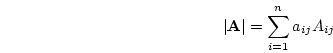 is the vector of parameters,
  is the vector of observed
statistics, and
is the vector of observed
statistics, and 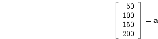 is the matrix of weights such that element
  gives the coefficient of parameter
  in equation
  . Then, if the
inverse of exists, the model is
identified. Thus in our example we have:
. Then, if the
inverse of exists, the model is
identified. Thus in our example we have:
 |
(36) |
where 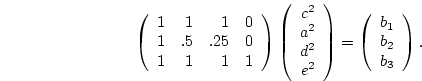 is Cov(MZ),
  is Cov(DZ), and
  is
is  . Now, what we would really like to find here is the left
inverse,
. Now, what we would really like to find here is the left
inverse,  , of such that
 . However, it
is easy to show that left inverses may exist only when has at
least as many rows as it does columns (for proof see, e.g., Searle,
1982, p. 147). Therefore, if we are limited to data from a classical
twin study, i.e. MZ and DZ twins reared together, it is necessary to
assume that one of the parameters
. However, it
is easy to show that left inverses may exist only when has at
least as many rows as it does columns (for proof see, e.g., Searle,
1982, p. 147). Therefore, if we are limited to data from a classical
twin study, i.e. MZ and DZ twins reared together, it is necessary to
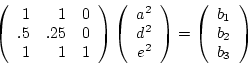
assume that one of the parameters  or
or  is zero to identify the
model. Let us suppose that we have reason to believe that
is zero to identify the
model. Let us suppose that we have reason to believe that  can be
ignored, so that the equations may be rewritten as:
can be
ignored, so that the equations may be rewritten as:
and in this case, the inverse of exists![[*]](footnote.png) . Another, generally superior, approach to resolving the
parameters of the model is to collect new data. For example, if we
collected data from separated MZ or DZ twins, then we could add a
fourth row to in equation 5.11 to get (for MZ
twins apart)
. Another, generally superior, approach to resolving the
parameters of the model is to collect new data. For example, if we
collected data from separated MZ or DZ twins, then we could add a
fourth row to in equation 5.11 to get (for MZ
twins apart)
 |
(37) |
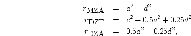
where 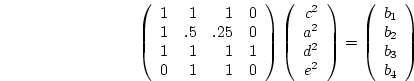 is Cov(MZA), and again the inverse of exists. Now it is not necessarily
the case that adding another type of relative (or type of rearing
environment) will turn an underidentified model into one that is
identified! Far from it, in fact, as we show with reference to
siblings reared together, and half-siblings and cousins reared apart.
Under our simple genetic model, the expected covariances of the
siblings and half-siblings are
is Cov(MZA), and again the inverse of exists. Now it is not necessarily
the case that adding another type of relative (or type of rearing
environment) will turn an underidentified model into one that is
identified! Far from it, in fact, as we show with reference to
siblings reared together, and half-siblings and cousins reared apart.
Under our simple genetic model, the expected covariances of the
siblings and half-siblings are
as could be shown by extending the methods outlined in
Chapter 3. In matrix form the equations are:
 |
(42) |
where is Cov(Sibs), is Cov(Half-sibs),
is Cov(Cousins), and is . Now in this
case, although we have as many types of relationship with different
expected covariance as there are unknown parameters in the model, we
still cannot identify all the parameters, because the matrix
is singular. The presence of data collected from cousins does not add
any information to the system, because their expected covariance is
exactly half that of the half-siblings. In general, if any row
(column) of a matrix can be expressed as a linear combination of the
other rows (columns) of a matrix, then the matrix is singular and
cannot be inverted. Note, however, that just because we cannot
identify the model as a whole, it does not mean that none of the
parameters can be estimated. In this example, we can obtain a valid
estimate of additive genetic variance  simply from, say, eight
times the difference of the half-sib and cousin covariances. With
this knowledge and the observed full sibling covariance, we could
estimate the combined effect of dominance and the shared
environment, but it is impossible to separate these two sources.
Throughout the above examples, we have taken advantage of their
inherent simplicity. The first useful feature is that the parameters
of the model only occur in linear combinations, so that, e.g., terms
of the form
simply from, say, eight
times the difference of the half-sib and cousin covariances. With
this knowledge and the observed full sibling covariance, we could
estimate the combined effect of dominance and the shared
environment, but it is impossible to separate these two sources.
Throughout the above examples, we have taken advantage of their
inherent simplicity. The first useful feature is that the parameters
of the model only occur in linear combinations, so that, e.g., terms
of the form 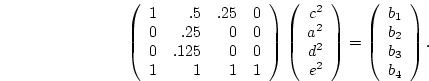 are not present. While true of a number of simple
genetic models that we shall use in this book, it is not the case for
them all (see Table
are not present. While true of a number of simple
genetic models that we shall use in this book, it is not the case for
them all (see Table ![[*]](crossref.png) for example). Nevertheless, some
insight may be gained by examining the model in this way, since if we
are able to identify both and then both parameters may be
estimated. Yet for complex systems this can prove a difficult task,
so we suggest an alternative, numerical approach.
The idea is to simulate
expected covariances for certain values of the parameters, and then
see whether a program such as Mx can recover these values from a
number of different starting points. If we find another set of
parameter values that generates the same expected variances and
covariances, the model is not identified. We shall not go into this
procedure in detail here, but simply note that it is very similar to
that described for power calculations in Chapter 7.
for example). Nevertheless, some
insight may be gained by examining the model in this way, since if we
are able to identify both and then both parameters may be
estimated. Yet for complex systems this can prove a difficult task,
so we suggest an alternative, numerical approach.
The idea is to simulate
expected covariances for certain values of the parameters, and then
see whether a program such as Mx can recover these values from a
number of different starting points. If we find another set of
parameter values that generates the same expected variances and
covariances, the model is not identified. We shall not go into this
procedure in detail here, but simply note that it is very similar to
that described for power calculations in Chapter 7.
Next: 8 Summary
Up: 5 Path Analysis and
Previous: 2 Variance Components Model:
Index
Jeff Lessem
2002-03-21