


Next: 2 Body Mass Index
Up: 2 Fitting Genetic Models
Previous: 2 Fitting Genetic Models
Index
1 Basic Genetic Model
Derivations of the expected variances and covariances of relatives
under a simple univariate genetic model have been reviewed briefly in the chapters on biometrical
genetics and path analysis (Chapters 3 and 5).
In brief, from biometrical genetic theory we can write structural
equations relating the phenotypes,  , of relatives
  and
and  (e.g., BMI values of first and second members of twin pairs) to their
underlying genotypes and environments which are latent variables whose
influence we must infer. We may decompose the total genetic effect on
a phenotype into contributions of:
(e.g., BMI values of first and second members of twin pairs) to their
underlying genotypes and environments which are latent variables whose
influence we must infer. We may decompose the total genetic effect on
a phenotype into contributions of:
- Additive effects of alleles at multiple loci (A),
- Dominance effects at multiple loci (D),
- Higher-order epistatic interactions between pairs
of loci (additive
 additive, additive dominance,
dominance dominance: AA, AD, DD), and so on.
additive, additive dominance,
dominance dominance: AA, AD, DD), and so on.
In practice even additive dominance and dominance
dominance epistasis are confounded with dominance in studies of
humans, and the power of resolving genetic dominance and additive
additive epistasis is very low. We shall therefore limit our
consideration to additive and dominance genetic effects.
Similarly, we may decompose the total environmental effect into that
due to environmental influences shared by twins or sibling pairs
reared in the same family (shared, common, or
between-family environmental ( ) effects), and that due to
environmental effects that make family members differ from one
another (within-family, specific, or random environmental
(
) effects), and that due to
environmental effects that make family members differ from one
another (within-family, specific, or random environmental
( ) effects). Thus, the observed phenotypes,
  and
and  ,
will be linear functions of the underlying additive genetic deviations
(
,
will be linear functions of the underlying additive genetic deviations
( and
and  ), dominance genetic deviations (
 and
and
 ), shared environmental deviations (
 and
and  ), and
random environmental deviations (
), and
random environmental deviations ( and
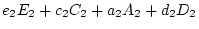
and  ). Assuming all
variables are scaled as deviations from zero, we have
). Assuming all
variables are scaled as deviations from zero, we have
In most models we do not expect the magnitude of genetic effects, or
the environmental effects, to differ between first and second twins,
so we set
 . Likewise, we do not expect the values of
 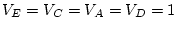 , and
, and  to vary as a function of relationship. In other words, the
effects of genotype and environment on the phenotype are the same
regardless of whether one is an MZ twin, a DZ twin, or not a twin at
all. In matrix form, we may write
to vary as a function of relationship. In other words, the
effects of genotype and environment on the phenotype are the same
regardless of whether one is an MZ twin, a DZ twin, or not a twin at
all. In matrix form, we may write
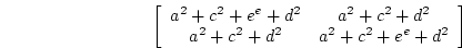
As shown in Chapter 5, this model generates a predicted
covariance matrix (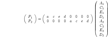 ) which is equal to
Unless two or more waves of measurement are used, or several variables
index the phenotype under study, residual
effects (such as measurement error)
will form part of the random environmental component, and are not
explicitly included in the model.
To obtain estimates for the genetic and environmental effects in this
model, we must also specify the variances and covariances among the
latent genetic and environmental factors. Two alternative
parameterizations are possible: 1) the variance components approach
(Chapter 3), or 2) the path coefficients model
(Chapter 5). The variance components approach becomes
cumbersome for designs involving more complex pedigree structures than
pairs of relatives, but it does have some numerical advantages (see
Chapter ![[*]](crossref.png) , p. ).
In the variance components approach we estimate variances of the latent non-shared and shared
environmental and additive and dominance genetic variables,
, p. ).
In the variance components approach we estimate variances of the latent non-shared and shared
environmental and additive and dominance genetic variables,  ,
,
 ,
,  , or
, or  , and fix
 . Thus, the
phenotypic variance is simply the sum of the four variance
components. In the path
coefficients approach we standardize the variances of the latent
variables to unity ( = = = =1) and estimate a
combination of
. Thus, the
phenotypic variance is simply the sum of the four variance
components. In the path
coefficients approach we standardize the variances of the latent
variables to unity ( = = = =1) and estimate a
combination of  , and as free parameters. Thus, the
phenotypic variance is a weighted sum of standardized variables. In
this volume we will often refer to models that have particular combinations of
free parameters in the general path coefficients model. Specifically,
we refer to an ACE model as one having only
additive genetic, common environment, and random environment effects;
an ADE model as one having additive genetic,
dominance, and random environment effects; an AE model as one having additive genetic and random environment
effects, and so on.
Figures 5.3a and 5.3b in Chapter 5
represent path diagrams for the two alternative parameterizations of
the full basic genetic model, illustrated for the case of pairs of
monozygotic twins (MZ) or dizygotic twins (DZ), who may be reared
together (MZT, DZT) or reared apart (MZA, DZA). For simplicity, we
make certain strong assumptions in this chapter, which are implied by
the way we have drawn the path diagrams in Figure 5.3:
, and as free parameters. Thus, the
phenotypic variance is a weighted sum of standardized variables. In
this volume we will often refer to models that have particular combinations of
free parameters in the general path coefficients model. Specifically,
we refer to an ACE model as one having only
additive genetic, common environment, and random environment effects;
an ADE model as one having additive genetic,
dominance, and random environment effects; an AE model as one having additive genetic and random environment
effects, and so on.
Figures 5.3a and 5.3b in Chapter 5
represent path diagrams for the two alternative parameterizations of
the full basic genetic model, illustrated for the case of pairs of
monozygotic twins (MZ) or dizygotic twins (DZ), who may be reared
together (MZT, DZT) or reared apart (MZA, DZA). For simplicity, we
make certain strong assumptions in this chapter, which are implied by
the way we have drawn the path diagrams in Figure 5.3:
- No genotype-environment correlation, i.e., latent genetic
variables
 are uncorrelated with latent environmental variables
and ;
are uncorrelated with latent environmental variables
and ;
- No genotype environment interaction, so that the
observed phenotypes are a linear function of the underlying genetic
and environmental variables;
- Random mating, i.e., no tendency for like
to marry like, an assumption which is implied by fixing the
covariance of the additive genetic deviations of DZ twins or full
sibs to
 ;
;
- Random placement of adoptees, so that the rearing environments
of separated twin pairs are uncorrelated.
We discuss ways in which these assumptions may be relaxed in
subsequent chapters, particularly Chapter 9 and
Chapter .
Next: 2 Body Mass Index
Up: 2 Fitting Genetic Models
Previous: 2 Fitting Genetic Models
Index
Jeff Lessem
2002-03-21