


Next: 6 Interpreting Univariate Results
Up: 2 Fitting Genetic Models
Previous: 4 Interpreting the Mx
Index
5 Building a Variance Components Model Mx Script
We include the variance components parameterization of the basic
structural equation model for completeness. It will not be developed
and applied in as great detail as the path coefficients
parameterization because (i) it is difficult to generalize to more
complex pedigree structures or multivariate problems, and (ii) doing
so would contribute much by weight but little by insight to this
volume. Readers seeking an easy introduction to twin models in Mx
may skip this section and focus their attention on
Section 6.2.3, the path coefficients parameterization.
For MZ and DZ twin pairs reared in the same family, the variance
components parameterization is presented in (Figure 5.3b).
Under the simplifying assumptions of the present chapter, the  expected covariance matrix of twin pairs (
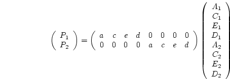 ) will be, in terms
of variance components,
) will be, in terms
of variance components,
where  is 1 for twins, full sibs or adoptees reared in the
same household, but 0 for separated twins or other biological
relatives reared apart;
is 1 for twins, full sibs or adoptees reared in the
same household, but 0 for separated twins or other biological
relatives reared apart;  is 1 for MZ twin pairs, 0.5 for DZ
pairs, full sibs, or parents and offspring, and 0 for genetically
unrelated individuals; and
is 1 for MZ twin pairs, 0.5 for DZ
pairs, full sibs, or parents and offspring, and 0 for genetically
unrelated individuals; and  is 1 for MZ pairs, 0.25 for DZ
pairs or full sibs, and 0 for most other relationships. In terms of
path coefficients, we need only substitute
is 1 for MZ pairs, 0.25 for DZ
pairs or full sibs, and 0 for most other relationships. In terms of
path coefficients, we need only substitute
 , and
, and 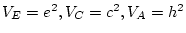 .
In data on twin pairs reared together the effects of shared
environment and genetic dominance are confounded. If both additive
genetic effects and shared environmental effects contribute to
variation in a trait, the covariance of DZ twin pairs will be less
than the MZ covariance, but greater than one-half the MZ covariance.
If both additive genetic effects and dominance genetic effects
contribute to variation in a trait, the covariance of DZ pairs will be
less than one-half the MZ covariance. In terms of variance
components, therefore, a substantial dominance genetic effect will
lead to a negative estimate of the shared environmental variance
component, if a model allowing for additive genetic and shared
environmental variance components is fitted; while conversely a
substantial shared environmental effect will lead to a negative
estimate of the dominance genetic variance component, if a model
allowing for additive and dominance genetic variance components is
fitted (Martin et al., 1978).
In terms of path coefficients, however, since we are
estimating parameters
.
In data on twin pairs reared together the effects of shared
environment and genetic dominance are confounded. If both additive
genetic effects and shared environmental effects contribute to
variation in a trait, the covariance of DZ twin pairs will be less
than the MZ covariance, but greater than one-half the MZ covariance.
If both additive genetic effects and dominance genetic effects
contribute to variation in a trait, the covariance of DZ pairs will be
less than one-half the MZ covariance. In terms of variance
components, therefore, a substantial dominance genetic effect will
lead to a negative estimate of the shared environmental variance
component, if a model allowing for additive genetic and shared
environmental variance components is fitted; while conversely a
substantial shared environmental effect will lead to a negative
estimate of the dominance genetic variance component, if a model
allowing for additive and dominance genetic variance components is
fitted (Martin et al., 1978).
In terms of path coefficients, however, since we are
estimating parameters  or
or  ,
,  or
or  can never take
negative values, and so we will obtain an estimate of
can never take
negative values, and so we will obtain an estimate of  in the
presence of dominance, or
in the
presence of dominance, or  in the presence of shared
environmental effects. Additional data on separated twin pairs
(Jinks and Fulker, 1970)
or on the parents or other relatives of twins
(Fulker, 1982; Heath,
1983) are needed to resolve the effects of
shared environment and genetic dominance when both are present.
Appendix
in the presence of shared
environmental effects. Additional data on separated twin pairs
(Jinks and Fulker, 1970)
or on the parents or other relatives of twins
(Fulker, 1982; Heath,
1983) are needed to resolve the effects of
shared environment and genetic dominance when both are present.
Appendix ![[*]](crossref.png) illustrates an example script for fitting a
variance components model to twin pair covariance matrices for two
like-sex twin pair groups. We estimate additive genetic, dominance
genetic and random environmental variance components in the matrices
illustrates an example script for fitting a
variance components model to twin pair covariance matrices for two
like-sex twin pair groups. We estimate additive genetic, dominance
genetic and random environmental variance components in the matrices
A, D and E. The covariance statement is the same
as for the path model example. The only change is in the calculation
group, which does not square the estimates to construct A, C, E and D.
For the young male like-sex pairs, the estimates are  ,
,  ,
and
,
and  . We can calculate standardized variance components by
hand, as
. We can calculate standardized variance components by
hand, as
 ,
,
 , and
, and
 , where
 (which can
be read directly from the variance in the expected covariance matrix).
In this example, random environmental effects account for 20.3% of
the variance, additive genetic effects for 36.4% of the variance, and
dominance genetic effects for 43.3% of the variance of BMI in young
adult males. By
(which can
be read directly from the variance in the expected covariance matrix).
In this example, random environmental effects account for 20.3% of
the variance, additive genetic effects for 36.4% of the variance, and
dominance genetic effects for 43.3% of the variance of BMI in young
adult males. By 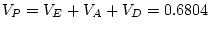 test of goodness-of-fit, our model gives
only a marginally acceptable fit to the data (
test of goodness-of-fit, our model gives
only a marginally acceptable fit to the data (
 ).
).
Next: 6 Interpreting Univariate Results
Up: 2 Fitting Genetic Models
Previous: 4 Interpreting the Mx
Index
Jeff Lessem
2002-03-21