


Next: 7 Testing the Equality
Up: 2 Fitting Genetic Models
Previous: 5 Building a Variance
Index
6 Interpreting Univariate Results
In model-fitting to univariate twin data, whether we use a variance
components or a path coefficients model, we are essentially testing
the following hypotheses:
- No family resemblance (``E'' model:
 :
:  )
)
- Family resemblance solely due to additive genetic effects
(``AE'' model:
 )
)
- Family resemblance solely due to shared environmental effects
(``CE'' model:
 )
)
- Family resemblance due to additive genetic plus
dominance genetic effects (``ADE'' model:
 )
)
- Family resemblance due to additive genetic plus shared
environmental effects (``ACE'' model:
 ).
).
Note that we never fit a model that excludes random environmental
effects, because it predicts perfect MZ twin pair correlations, which
in turn generate a singular expected covariance matrix![[*]](footnote.png) . From inspection of the
twin pair correlations for BMI, we noted that they were most
consistent with a model allowing for additive genetic, dominance
genetic, and random environmental effects. Model-fitting gives three
important advantages at this stage:
. From inspection of the
twin pair correlations for BMI, we noted that they were most
consistent with a model allowing for additive genetic, dominance
genetic, and random environmental effects. Model-fitting gives three
important advantages at this stage:
- An overall test of the goodness of fit of the model
- A test of the relative goodness of fit of different models, as
assessed by likelihood-ratio
 . For example, we can test
whether the fit is significantly worse if we omit genetic dominance
for BMI
. For example, we can test
whether the fit is significantly worse if we omit genetic dominance
for BMI
- Maximum-likelihood parameter estimates under the best-fitting
model.
Table 6.4 tabulates goodness-of-fit chi-squares obtained in four
Table 6.4:
Results of fitting models to twin pairs
covariance matrices for Body Mass Index: Two-group analyses,
complete pairs only.
| |
Females |
Males |
| |
Young |
Older |
Young |
Older |
| Model (d.f.) |
|
 |
|
|
|
|
|
|
| CE (4) |
160.72 |
 .001 .001 |
87.36 |
.001 |
97.20 |
.001 |
37.14 |
.001 |
| AE (4) |
8.06 |
.09 |
2.38 |
.67 |
10.88 |
.03 |
5.03 |
.28 |
| ACE (3) |
8.06 |
.05 |
2.38 |
.50 |
10.88 |
.01 |
5.03 |
.17 |
| ADE (3) |
3.71 |
.29 |
1.97 |
.58 |
7.28 |
.06 |
5.03 |
.17 |
separate analyses of the data from younger or older, female or male
like-sex twin pairs. Let us consider the results for young females
first. The non-genetic model (CE) yields a
chi-squared of 160.72 for 4 degrees of freedom, which is highly significant and implies a
very poor fit to the data indeed. In stark contrast, the alternative
model of additive genes and random environment (AE) is not rejected by
the data, but fits moderately well ( ). Adding common
environmental effects (the ACE model) does not improve the fit
whatsoever, but the loss of a degree of freedom makes the
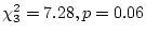
significant at the .05 level. Finally, the ADE model which
substitutes genetic dominance for common environmental effects, fits
the best according to the probability level. We can test whether the
dominance variation is significant by using the likelihood ratio test.
The difference
between the of a general model (
). Adding common
environmental effects (the ACE model) does not improve the fit
whatsoever, but the loss of a degree of freedom makes the
significant at the .05 level. Finally, the ADE model which
substitutes genetic dominance for common environmental effects, fits
the best according to the probability level. We can test whether the
dominance variation is significant by using the likelihood ratio test.
The difference
between the of a general model ( ) and the that of a
submodel (
) and the that of a
submodel ( ) is itself a and has
 degrees of freedom (where subscripts
  and
and
 respectively refer to the submodel and general model, in other words,
the difference in df between the general model and the submodel). In this
case, comparing the AE and the ADE model gives a likelihood ratio
of
respectively refer to the submodel and general model, in other words,
the difference in df between the general model and the submodel). In this
case, comparing the AE and the ADE model gives a likelihood ratio
of
 with
with  df. This is significant at
the .05 level, so we say that there is significant deterioration in
the fit of the model when the parameter
df. This is significant at
the .05 level, so we say that there is significant deterioration in
the fit of the model when the parameter  is fixed to zero, or
simply that the parameter is significant.
Now we are in a position to compare the results of model-fitting in
females and males, and in young and older twins. In each case, a
non-genetic (CE) model yields a significant chi-squared, implying a
very poor fit to the data: the deviations of the observed covariance
matrices from the expected covariance matrices under the
maximum-likelihood parameter estimates are highly significant. In all
groups, a full model allowing for additive plus dominance genetic
effects and random environmental effects (ADE) gives an acceptable fit
to the data, although in the case of young males the fit is somewhat
marginal. In the two older cohorts, however, a model which allows for
only additive genetic plus random environmental effects (AE) does
not give a significantly worse fit than the full (ADE) model, by
likelihood-ratio test. In older females, for example, the
likelihood-ratio chi-square is
is fixed to zero, or
simply that the parameter is significant.
Now we are in a position to compare the results of model-fitting in
females and males, and in young and older twins. In each case, a
non-genetic (CE) model yields a significant chi-squared, implying a
very poor fit to the data: the deviations of the observed covariance
matrices from the expected covariance matrices under the
maximum-likelihood parameter estimates are highly significant. In all
groups, a full model allowing for additive plus dominance genetic
effects and random environmental effects (ADE) gives an acceptable fit
to the data, although in the case of young males the fit is somewhat
marginal. In the two older cohorts, however, a model which allows for
only additive genetic plus random environmental effects (AE) does
not give a significantly worse fit than the full (ADE) model, by
likelihood-ratio test. In older females, for example, the
likelihood-ratio chi-square is
 , with degrees of
freedom equal to , i.e.,
, with degrees of
freedom equal to , i.e.,
 with probability
 ; while in older males we have
 .
For the older cohorts, therefore, we find no significant evidence for
genetic dominance. In young adults, however, significant dominance is
observed in females (as noted above) and the dominance genetic effect
is almost significant in males (
.
For the older cohorts, therefore, we find no significant evidence for
genetic dominance. In young adults, however, significant dominance is
observed in females (as noted above) and the dominance genetic effect
is almost significant in males (
 ).
Table 6.5 summarizes
).
Table 6.5 summarizes
Table 6.5:
Standardized parameter estimates under
best-fitting model. Two-group analyses, complete pairs only.
| |
Estimate |
| |
a |
c |
e |
d |
| Young females |
0.40 |
0 |
0.22 |
0.38 |
| Older females |
0.69 |
0 |
0.31 |
0 |
| Young males |
0.36 |
0 |
0.20 |
0.44 |
| Older males |
0.70 |
0 |
0.30 |
0 |
variance component estimates under the best-fitting models.
Random environment accounts for a relatively modest proportion of
the total variation in BMI, but appears to be having a larger effect
in older than in younger individuals (30-31% versus 20-22%).
Although the estimate of the narrow heritability
(i.e., proportion of the total variance
accounted for by additive genetic factors) is higher in the older
cohort (69-70% vs 36-40%), the broad heritability
(additive plus non-additive genetic
variance) is higher in the young twins (78-80%).
Next: 7 Testing the Equality
Up: 2 Fitting Genetic Models
Previous: 5 Building a Variance
Index
Jeff Lessem
2002-03-21